In this vignette we provide details on transforming data into a format suitable to fit piece-wise exponential (additive) models (PAM). Three main cases need to be distinguished
Standard time-to-event data
In the case of “standard” time-to-event the data, the transformation
is relatively straight forward and handled by the as_ped
(as piece-wise
exponential data) function. This
function internally calls survival::survSplit, thus all
arguments available for the survSplit function are also
available to the as_ped function.
Using defaults
As an example data set we first consider a data set of a stomach area
tumor available from the pammtools
package. Patients were operated on to remove the tumor. Some patients
experienced complications during the operation:
data("tumor")
tumor <- tumor %>%
  mutate(id = row_number()) %>%
  select(id, everything())
head(tumor)
## # A tibble: 6 × 10
## id days status charlson_score age sex transfusion complications
## <int> <dbl> <int> <int> <int> <fct> <fct> <fct>
## 1 1 579 0 2 58 female yes no
## 2 2 1192 0 2 52 male no yes
## 3 3 308 1 2 74 female yes no
## 4 4 33 1 2 57 male yes yes
## 5 5 397 1 2 30 female yes no
## 6 6 1219 0 2 66 female yes no
## # ℹ 2 more variables: metastases <fct>, resection <fct>Each row contains information on the survival time
(days), an event indicator (status) as well as
information about comorbidities (charlson_score),
age, sex, and covariates that might be
relevant like whether or not complications occurred
(complications) and whether the cancer metastasized
(metastases).
To transform the data into piece-wise exponential data
(ped) format, we need to
define interval break points
create pseudo-observations for each interval in which subject was under risk.
Using the pammtools package this is easily achieved with
the as_ped function as follows:
ped <- as_ped(Surv(days, status) ~ ., data = tumor, id = "id")
ped %>% filter(id %in% c(132, 141, 145)) %>%
  select(id, tstart, tend, interval, offset, ped_status, age, sex, complications)
## id tstart tend interval offset ped_status age sex complications
## 1 132 0 1 (0,1] 0.0000000 0 78 male yes
## 2 132 1 2 (1,2] 0.0000000 0 78 male yes
## 3 132 2 3 (2,3] 0.0000000 0 78 male yes
## 4 132 3 5 (3,5] 0.6931472 1 78 male yes
## 5 141 0 1 (0,1] 0.0000000 0 79 male yes
## 6 141 1 2 (1,2] 0.0000000 0 79 male yes
## 7 141 2 3 (2,3] 0.0000000 0 79 male yes
## 8 141 3 5 (3,5] 0.6931472 0 79 male yes
## 9 141 5 6 (5,6] 0.0000000 0 79 male yes
## 10 141 6 7 (6,7] 0.0000000 0 79 male yes
## 11 141 7 8 (7,8] 0.0000000 0 79 male yes
## 12 141 8 10 (8,10] 0.6931472 0 79 male yes
## 13 141 10 11 (10,11] 0.0000000 0 79 male yes
## 14 141 11 12 (11,12] 0.0000000 0 79 male yes
## 15 141 12 13 (12,13] 0.0000000 0 79 male yes
## 16 141 13 14 (13,14] 0.0000000 1 79 male yes
## 17 145 0 1 (0,1] 0.0000000 0 60 male yes
## 18 145 1 2 (1,2] 0.0000000 0 60 male yes
## 19 145 2 3 (2,3] 0.0000000 0 60 male yes
## 20 145 3 5 (3,5] 0.6931472 0 60 male yes
## 21 145 5 6 (5,6] 0.0000000 0 60 male yes
## 22 145 6 7 (6,7] 0.0000000 0 60 male yes
## 23 145 7 8 (7,8] 0.0000000 1 60 male yesWhen no cut points are specified, the default is to use the unique
event times. As can be seen from the above output, the function creates
an id variable, indicating the subjects
,
with one row per interval that the subject “visited”. Thus,
- subject
132was at risk during 4 intervals, - subject
141was at risk during 12 intervals, - and subject
145in 7 intervals.
In addition to the optional id variable the function
also creates
-
tstart: the beginning of each interval -
tend: the end of each interval -
interval: a factor variable denoting the interval -
offset: the log of the duration during which the subject was under risk in that interval
Additionally the time-constant covariates (here: age,
sex, complications,) are repeated
number of times, where
is the number of intervals during which subject
was in the risk set.
Custom cut points
Per default, the as_ped function uses all unique event
times as cut points (which is a sensible default as for example the
(cumulative) baseline hazard estimates in Cox-PH functions are also
updated at event times). Also, PAMMs represent the baseline hazard via
splines whose basis functions are evaluated at the cut points. Using
unique events times automatically increases the density of cut points in
relevant areas of the follow-up.
In some cases, however, one might want to reduce the number of cut
points, to reduce the size of the resulting data and/or faster
estimation times. To do so the cut argument has to be
specified. Following the above example, we can use only 4 cut points
,
resulting in
intervals:
ped2 <- as_ped(Surv(days, status) ~ ., data = tumor, cut = c(0, 3, 7, 15), id = "id")
ped2 %>%
  filter(id %in% c(132, 141, 145)) %>%
  select(id, tstart, tend, interval, offset, ped_status, age, sex, complications)
## id tstart tend interval offset ped_status age sex complications
## 1 132 0 3 (0,3] 1.0986123 0 78 male yes
## 2 132 3 7 (3,7] 0.6931472 1 78 male yes
## 3 141 0 3 (0,3] 1.0986123 0 79 male yes
## 4 141 3 7 (3,7] 1.3862944 0 79 male yes
## 5 141 7 15 (7,15] 1.9459101 1 79 male yes
## 6 145 0 3 (0,3] 1.0986123 0 60 male yes
## 7 145 3 7 (3,7] 1.3862944 0 60 male yes
## 8 145 7 15 (7,15] 0.0000000 1 60 male yesNote that now subjects 141 and 145 have
both three rows in the data set. The fact that subject 141
was in the risk set of the last interval for a longer time than subject
145 is, however, still accounted for by the
offset variable. Note that the offset for
subject 145 is only 0, because the last
interval for this subject starts at
and the subject experienced and event at
,
thus
## # A tibble: 2 × 10
##      id  days status charlson_score   age sex    transfusion complications
##   <int> <dbl>  <int>          <int> <int> <fct>  <fct>       <fct>
## 1    85   126      1              2    64 female yes         no
## 2   112   888      0              5    71 male   yes         no
## # ℹ 2 more variables: metastases <fct>, resection <fct>
Left-truncated Data
In left truncated data, subjects enter the risk set at some time-point unequal to zero. Such data usually ships in the so called start-stop notation, where for each subject the start time specifies the left-truncation time (can also be 0) and the stop time the time-to-event, which can be right-censored.
For an illustration, we use a data set on infant mortality and
maternal death available in the eha
package (see ?eha::infants) for details.
##   stratum enter exit event mother age  sex      parish   civst    ses year
## 1       1    55  365     0   dead  26  boy Nedertornea married farmer 1877
## 2       1    55  365     0  alive  26  boy Nedertornea married farmer 1870
## 3       1    55  365     0  alive  26  boy Nedertornea married farmer 1882
## 4       2    13   76     1   dead  23 girl Nedertornea married  other 1847
## 5       2    13  365     0  alive  23 girl Nedertornea married  other 1847
## 6       2    13  365     0  alive  23 girl Nedertornea married  other 1848
As children were included in the study after death of their mother,
their survival time is left-truncated at the entry time (variable
enter). When transforming such data to the PED format, we
need to create a interval cut-point at each entry time. In general, each
interval has to be constructed such that only subjects already at risk
have an entry in the PED data. The previously introduced function
as_ped can be also used for this setting, however, the LHS
of the formula must be in start-stop format:
infants_ped <- as_ped(Surv(enter, exit, event) ~ mother + age, data = infants)
infants_ped %>% filter(id == 4)
## id tstart tend interval offset ped_status mother age
## 1 4 13 14 (13,14] 0.0000000 0 dead 23
## 2 4 14 16 (14,16] 0.6931472 0 dead 23
## 3 4 16 17 (16,17] 0.0000000 0 dead 23
## 4 4 17 18 (17,18] 0.0000000 0 dead 23
## 5 4 18 22 (18,22] 1.3862944 0 dead 23
## 6 4 22 24 (22,24] 0.6931472 0 dead 23
## 7 4 24 28 (24,28] 1.3862944 0 dead 23
## 8 4 28 29 (28,29] 0.0000000 0 dead 23
## 9 4 29 30 (29,30] 0.0000000 0 dead 23
## 10 4 30 31 (30,31] 0.0000000 0 dead 23
## 11 4 31 36 (31,36] 1.6094379 0 dead 23
## 12 4 36 39 (36,39] 1.0986123 0 dead 23
## 13 4 39 44 (39,44] 1.6094379 0 dead 23
## 14 4 44 53 (44,53] 2.1972246 0 dead 23
## 15 4 53 55 (53,55] 0.6931472 0 dead 23
## 16 4 55 62 (55,62] 1.9459101 0 dead 23
## 17 4 62 76 (62,76] 2.6390573 1 dead 23For analysis of such data refer to the Left-truncation vignette
Data with time-dependent covariates
In case of data with time-dependent covariates (that should not be modeled as cumulative effects), the follow-up is usually split at desired cut-points and additionally at the time-points at which the TDC changes its value.
We assume that the data is provided in two data sets, one that contains time-to-event data and time-constant covariates and one data set that contains information of time-dependent covariates.
For illustration, we use the pbc data from the
survival package. Before the actual data transformation we
perform the data preprocessing in
vignette("timedep", package="survival"):
data("pbc", package = "survival") # loads pbc and pbcseq
pbc <- pbc %>% filter(id <= 312) %>%
  mutate(status = 1L * (status == 2)) %>%
  select(id:sex, bili, protime)
We want to transform the data such that we could fit a concurrent
effect of the time-dependent covariates bili and
protime, therefore, the RHS of the formula passed to
as_ped needs to contain an additional component, separated
by | and all variables for which should be transformed to
the concurrent format specified within the concurrent
special. The data sets are provided within a list. In
concurrent, we also have to specify the name of the
variable which stores information on the time points at which the TDCs
are updated.
ped_pbc <- as_ped(
  data    = list(pbc, pbcseq),
  formula = Surv(time, status) ~ . + concurrent(bili, protime, tz_var = "day"),
  id      = "id")
Multiple data sets can be provided within the list and multiple
concurrent terms with different tz_var
arguments can be specified with different lags. This will increase the
data set, as an (additional) split point will be generated for each
(lagged) time-point at which the TDC was observed:
pbc_ped <- as_ped(data = list(pbc, pbcseq),
  formula = Surv(time, status) ~ . + concurrent(bili, tz_var = "day") +
    concurrent(protime, tz_var = "day", lag = 10),
    id = "id")
If different tz_var arguments are provided, the union of
both will be used as cut points in addition to usual cut points.
Warning: For time-points on the follow up that have no observation of the TDC, the last observation will be carried forward until the next update is available.
Data with time-dependent covariates (with cumulative effects)
Here we demonstrate data transformation of data with TDCs (, that subsequently will be modeled as cumulative effects defined as
Here
-
the three-variate function defines the so-called partial effects of the TDC observed at exposure time on the hazard at time (Bender et al. 2018). The general partial effect definition given above is only one possibility, other common choices are
-
(This is the WCE model by Sylvestre and
Abrahamowicz (2009))
-
(This is the DLNM model by Gasparrini et al.
(2017))
-
(This is the WCE model by Sylvestre and
Abrahamowicz (2009))
the cumulative effect at follow-up time is the integral (or sum) of the partial effects over exposure times contained within
the so called lag-lead window (or window of effectiveness) is denoted by . This represents the set of exposure times at which exposures can affect the hazard rate at time . The most common definition is , which means that all exposures that were observed prior to or at are eligible.
As before we use the function as_ped to transform the
data and additionally use the formula special cumulative
(for functional covariate) to specify
the partial effect structure on the right-hand side of the formula.
Let
(time) the follow up time,
(z1) and
(z2) two TDCs observed at different exposure time grids
(tz1) and
(tz2) with lag-lead windows
and
(defined by
ll2 <- function(t, tz) { t >= tz + 2}).
The table below gives a selection of possible partial effects and the
usage of cumulative to create matrices needed to estimate
different types of cumulative effects of
and
:
| partial effect |
as_ped specification |
|---|---|
cumulative(latency(tz1), z1, tz_var= "tz1") |
|
cumulative(time, latency(tz1), z1, tz_var="tz1") |
|
cumulative(time, tz1, z1, tz_var="tz1") |
|
cumulative(time, tz1, z1, tz_var="tz1") + cumulative(latency(tz2), z2, tz_var="tz2", ll_fun=ll2) |
|
| … | … |
Note that
the variable representing follow-up time in
cumulative(heretime) must match the time variable specified on the left-hand side of theformulathe variable representing exposure time (here
tz1andtz2) must be wrapped withinlatency()to tellas_pedto calculateby default, is defined as
function(t, tz) {t >= tz}, thus for it is not necessary to explicitly specify the lag-lead window. In case you want to use a custom lag-lead window, provide the respective function to thell_funargument incumulative(seell2in the examples above)cumulativemakes no difference between partial effects such as and as the necessary data transformation is the same in both cases. Later, however, when fitting the model, a distinction must be mademore than one variable can be provided to
cumulative, which can be convenient if multiple covariates should have the same time components and the same lag-lead windowmultiple
cumulativeterms can be specified, having different exposure timest_z,s_zand/or different lag-lead windows for different covariates ,To tell
cumulativewhich of the variables specified is the exposure time , thetz_varargument must be specified within eachcumulativeterm. The follow-up time component will be automatically recognized via the left-hand side of theformula.
One time-dependent covariate
For illustration we use the ICU patients data sets
patient and daily provided in the
pammtools package, with follow-up time
survhosp
(),
exposure time Study_Day
()
and TDCs caloriesPercentage
and proteinGproKG
():
head(patient)## Year CombinedicuID CombinedID Survdays PatientDied survhosp Gender Age
## 1 2007 1114 1110 30.1 0 30.1 Male 68
## 2 2007 1114 1111 30.1 0 30.1 Female 57
## 3 2007 1114 1116 9.8 1 9.8 Female 68
## 4 2007 598 1316 30.1 0 30.1 Male 47
## 5 2007 365 1410 30.1 0 30.1 Male 69
## 6 2007 365 1414 30.1 0 5.4 Male 47
## AdmCatID ApacheIIScore BMI DiagID2
## 1 Surgical Elective 20 31.60321 Cardio-Vascular
## 2 Medical 22 24.34176 Respiratory
## 3 Surgical Elective 25 17.99308 Cardio-Vascular
## 4 Medical 16 33.74653 Orthopedic/Trauma
## 5 Surgical Elective 20 38.75433 Respiratory
## 6 Medical 21 45.00622 Respiratory
head(daily)## # A tibble: 6 × 4
## CombinedID Study_Day caloriesPercentage proteinGproKG
## <int> <int> <dbl> <dbl>
## 1 1110 1 0 0
## 2 1110 2 0 0
## 3 1110 3 4.05 0
## 4 1110 4 35.1 0.259
## 5 1110 5 77.2 0.647
## 6 1110 6 17.3 0Below we illustrate the usage of as_ped and
cumulative to obtain covariate matrices for the latency
matrix of follow up time and exposure time and a matrix of the TDC
(caloriesPercentage). The follow up will be split in 30
intervals with interval breaks points 0:30. By default, the
exposure time provided to tz_var will be used as a suffix
for the names of the new matrix columns to indicate the exposure they
refer to, however, you can override the suffix by specifying the
suffix argument to cumulative.
ped <- as_ped(
  data    = list(patient, daily),
  formula = Surv(survhosp, PatientDied) ~ . +
    cumulative(latency(Study_Day), caloriesPercentage, tz_var = "Study_Day"),
  cut     = 0:30,
  id = "CombinedID")
str(ped, 1)
## Classes 'fped', 'ped' and 'data.frame': 37258 obs. of 18 variables:
## $ CombinedID : int 1110 1110 1110 1110 1110 1110 1110 1110 1110 1110 ...
## $ tstart : num 0 1 2 3 4 5 6 7 8 9 ...
## $ tend : int 1 2 3 4 5 6 7 8 9 10 ...
## $ interval : Factor w/ 30 levels "(0,1]","(1,2]",..: 1 2 3 4 5 6 7 8 9 10 ...
## $ offset : num 0 0 0 0 0 0 0 0 0 0 ...
## $ ped_status : num 0 0 0 0 0 0 0 0 0 0 ...
## $ Year : Factor w/ 4 levels "2007","2008",..: 1 1 1 1 1 1 1 1 1 1 ...
## $ CombinedicuID : Factor w/ 456 levels "21","24","25",..: 355 355 355 355 355 355 355 355 355 355 ...
## $ Survdays : num 30.1 30.1 30.1 30.1 30.1 30.1 30.1 30.1 30.1 30.1 ...
## $ Gender : Factor w/ 2 levels "Female","Male": 2 2 2 2 2 2 2 2 2 2 ...
## $ Age : int 68 68 68 68 68 68 68 68 68 68 ...
## $ AdmCatID : Factor w/ 3 levels "Medical","Surgical Elective",..: 2 2 2 2 2 2 2 2 2 2 ...
## $ ApacheIIScore : int 20 20 20 20 20 20 20 20 20 20 ...
## $ BMI : num 31.6 31.6 31.6 31.6 31.6 ...
## $ DiagID2 : Factor w/ 9 levels "Gastrointestinal",..: 2 2 2 2 2 2 2 2 2 2 ...
## $ Study_Day_latency : num [1:37258, 1:12] 0 0 1 2 3 4 5 6 7 8 ...
## $ caloriesPercentage: num [1:37258, 1:12] 0 0 0 0 0 0 0 0 0 0 ...
## ..- attr(*, "dimnames")=List of 2
## $ LL : num [1:37258, 1:12] 0 1 1 1 1 1 1 1 1 1 ...
## - attr(*, "breaks")= int [1:31] 0 1 2 3 4 5 6 7 8 9 ...
## - attr(*, "id_var")= chr "CombinedID"
## - attr(*, "intvars")= chr [1:6] "CombinedID" "tstart" "tend" "interval" ...
## - attr(*, "trafo_args")=List of 3
## - attr(*, "time_var")= chr "survhosp"
## - attr(*, "status_var")= chr "PatientDied"
## - attr(*, "func")=List of 1
## - attr(*, "ll_funs")=List of 1
## - attr(*, "tz")=List of 1
## - attr(*, "tz_vars")=List of 1
## - attr(*, "ll_weights")=List of 1
## - attr(*, "func_mat_names")=List of 1As you can see, the data is transformed to the PED format as before
and two additional matrix columns are added,
Study_Day_latency and
caloriesPercentage.
Two time-dependent covariates observed on the same exposure time grid
Using the same data, we show a slightly more complex example with two
functional covariate terms with partial effects
and
.
As in the case of ICU patient data, both TDCs were observed on the same
exposure time grid, we want to use the same lag-lead window and the
latency term
occurs in both partial effects, we only need to specify one
cumulative term.
ped <- as_ped(
  data = list(patient, daily),
  formula = Surv(survhosp, PatientDied) ~ . +
    cumulative(survhosp, latency(Study_Day), caloriesPercentage, proteinGproKG,
      tz_var = "Study_Day"),
  cut = 0:30,
  id = "CombinedID")
str(ped, 1)
## Classes 'fped', 'ped' and 'data.frame': 37258 obs. of 20 variables:
## $ CombinedID : int 1110 1110 1110 1110 1110 1110 1110 1110 1110 1110 ...
## $ tstart : num 0 1 2 3 4 5 6 7 8 9 ...
## $ tend : int 1 2 3 4 5 6 7 8 9 10 ...
## $ interval : Factor w/ 30 levels "(0,1]","(1,2]",..: 1 2 3 4 5 6 7 8 9 10 ...
## $ offset : num 0 0 0 0 0 0 0 0 0 0 ...
## $ ped_status : num 0 0 0 0 0 0 0 0 0 0 ...
## $ Year : Factor w/ 4 levels "2007","2008",..: 1 1 1 1 1 1 1 1 1 1 ...
## $ CombinedicuID : Factor w/ 456 levels "21","24","25",..: 355 355 355 355 355 355 355 355 355 355 ...
## $ Survdays : num 30.1 30.1 30.1 30.1 30.1 30.1 30.1 30.1 30.1 30.1 ...
## $ Gender : Factor w/ 2 levels "Female","Male": 2 2 2 2 2 2 2 2 2 2 ...
## $ Age : int 68 68 68 68 68 68 68 68 68 68 ...
## $ AdmCatID : Factor w/ 3 levels "Medical","Surgical Elective",..: 2 2 2 2 2 2 2 2 2 2 ...
## $ ApacheIIScore : int 20 20 20 20 20 20 20 20 20 20 ...
## $ BMI : num 31.6 31.6 31.6 31.6 31.6 ...
## $ DiagID2 : Factor w/ 9 levels "Gastrointestinal",..: 2 2 2 2 2 2 2 2 2 2 ...
## $ survhosp_mat : int [1:37258, 1:12] 0 1 2 3 4 5 6 7 8 9 ...
## $ Study_Day_latency : num [1:37258, 1:12] 0 0 1 2 3 4 5 6 7 8 ...
## $ caloriesPercentage: num [1:37258, 1:12] 0 0 0 0 0 0 0 0 0 0 ...
## ..- attr(*, "dimnames")=List of 2
## $ proteinGproKG : num [1:37258, 1:12] 0 0 0 0 0 0 0 0 0 0 ...
## ..- attr(*, "dimnames")=List of 2
## $ LL : num [1:37258, 1:12] 0 1 1 1 1 1 1 1 1 1 ...
## - attr(*, "breaks")= int [1:31] 0 1 2 3 4 5 6 7 8 9 ...
## - attr(*, "id_var")= chr "CombinedID"
## - attr(*, "intvars")= chr [1:6] "CombinedID" "tstart" "tend" "interval" ...
## - attr(*, "trafo_args")=List of 3
## - attr(*, "time_var")= chr "survhosp"
## - attr(*, "status_var")= chr "PatientDied"
## - attr(*, "func")=List of 1
## - attr(*, "ll_funs")=List of 1
## - attr(*, "tz")=List of 1
## - attr(*, "tz_vars")=List of 1
## - attr(*, "ll_weights")=List of 1
## - attr(*, "func_mat_names")=List of 1Multiple TDCs observed at different exposure time grids
To illustrate data transformation when TDCs
and
were observed on different exposure time grids
(
and
)
and are assumed to have different lag_lead windows
and
,
we use simulated data simdf_elra contained in
pammtools (see example in
sim_pexp for data generation).
simdf_elra## # A tibble: 250 × 9
## id time status x1 x2 tz1 z.tz1 tz2 z.tz2
## * <int> <dbl> <int> <dbl> <dbl> <list> <list> <list> <list>
## 1 1 3.22 1 1.59 4.61 <int [10]> <dbl [10]> <int [11]> <dbl [11]>
## 2 2 10 0 -0.530 0.178 <int [10]> <dbl [10]> <int [11]> <dbl [11]>
## 3 3 0.808 1 -2.43 3.25 <int [10]> <dbl [10]> <int [11]> <dbl [11]>
## 4 4 3.04 1 0.696 1.26 <int [10]> <dbl [10]> <int [11]> <dbl [11]>
## 5 5 3.36 1 2.54 3.71 <int [10]> <dbl [10]> <int [11]> <dbl [11]>
## 6 6 4.07 1 -0.0231 0.607 <int [10]> <dbl [10]> <int [11]> <dbl [11]>
## 7 7 0.534 1 1.68 1.74 <int [10]> <dbl [10]> <int [11]> <dbl [11]>
## 8 8 1.57 1 -1.89 2.51 <int [10]> <dbl [10]> <int [11]> <dbl [11]>
## 9 9 2.39 1 0.126 3.38 <int [10]> <dbl [10]> <int [11]> <dbl [11]>
## 10 10 6.61 1 1.79 1.06 <int [10]> <dbl [10]> <int [11]> <dbl [11]>
## # ℹ 240 more rows## Warning: `cols` is now required when using `unnest()`.
## ℹ Please use `cols = c(tz1)`.## # A tibble: 10 × 2
## id tz1
## <int> <int>
## 1 1 1
## 2 1 2
## 3 1 3
## 4 1 4
## 5 1 5
## 6 1 6
## 7 1 7
## 8 1 8
## 9 1 9
## 10 1 10## Warning: `cols` is now required when using `unnest()`.
## ℹ Please use `cols = c(tz2)`.## # A tibble: 11 × 2
## id tz2
## <int> <int>
## 1 1 -5
## 2 1 -4
## 3 1 -3
## 4 1 -2
## 5 1 -1
## 6 1 0
## 7 1 1
## 8 1 2
## 9 1 3
## 10 1 4
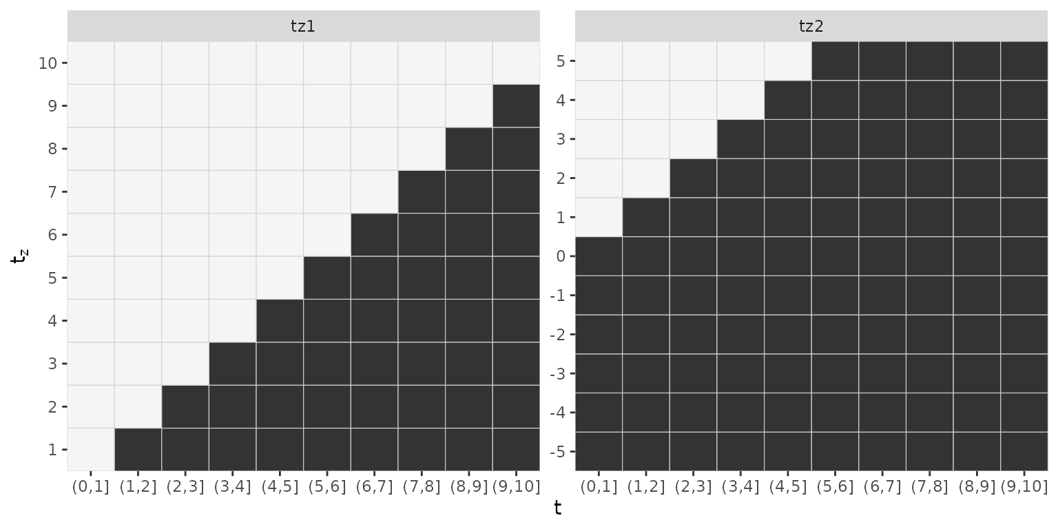
## 11 1 5Note that tz1 has a maximum length of 10, while
tz2 has a maximum length of 11 and while
tz1 was observed during the follow up, tz2 was
partially observed before the beginning of the follow up.
If we wanted to estimate the following cumulative effects
- and
with and the data transformation function must reflect the different exposure times as well as different lag-lead window specifications as illustrated below:
ped_sim <- as_ped(
  data = simdf_elra,
  formula = Surv(time, status) ~ . +
    cumulative(time, latency(tz1), z.tz1, tz_var = "tz1") +
    cumulative(latency(tz2), z.tz2, tz_var = "tz2"),
  cut = 0:10,
  id = "id")
str(ped_sim, 1)
## Classes 'fped', 'ped' and 'data.frame': 1004 obs. of 15 variables:
## $ id : int 1 1 1 1 2 2 2 2 2 2 ...
## $ tstart : num 0 1 2 3 0 1 2 3 4 5 ...
## $ tend : int 1 2 3 4 1 2 3 4 5 6 ...
## $ interval : Factor w/ 10 levels "(0,1]","(1,2]",..: 1 2 3 4 1 2 3 4 5 6 ...
## $ offset : num 0 0 0 -1.53 0 ...
## $ ped_status : num 0 0 0 1 0 0 0 0 0 0 ...
## $ x1 : num 1.59 1.59 1.59 1.59 -0.53 ...
## $ x2 : num 4.612 4.612 4.612 4.612 0.178 ...
## $ time_tz1_mat: int [1:1004, 1:10] 0 1 2 3 0 1 2 3 4 5 ...
## $ tz1_latency : num [1:1004, 1:10] 0 0 1 2 0 0 1 2 3 4 ...
## $ z.tz1_tz1 : num [1:1004, 1:10] -2.014 -2.014 -2.014 -2.014 -0.978 ...
## ..- attr(*, "dimnames")=List of 2
## $ LL_tz1 : num [1:1004, 1:10] 0 1 1 1 0 1 1 1 1 1 ...
## $ tz2_latency : num [1:1004, 1:11] 5 6 7 8 5 6 7 8 9 10 ...
## $ z.tz2_tz2 : num [1:1004, 1:11] -0.689 -0.689 -0.689 -0.689 0.693 ...
## ..- attr(*, "dimnames")=List of 2
## $ LL_tz2 : num [1:1004, 1:11] 1 1 1 1 1 1 1 1 1 1 ...
## - attr(*, "breaks")= int [1:11] 0 1 2 3 4 5 6 7 8 9 ...
## - attr(*, "id_var")= chr "id"
## - attr(*, "intvars")= chr [1:6] "id" "tstart" "tend" "interval" ...
## - attr(*, "trafo_args")=List of 3
## - attr(*, "time_var")= chr "time"
## - attr(*, "status_var")= chr "status"
## - attr(*, "func")=List of 2
## - attr(*, "ll_funs")=List of 2
## - attr(*, "tz")=List of 2
## - attr(*, "tz_vars")=List of 2
## - attr(*, "ll_weights")=List of 2
## - attr(*, "func_mat_names")=List of 2Note how the matrix covariates associated with tz1 have
10 columns while matrix covariates associated with tz2 have
11 columns. Note also that the lag-lead matrices differ
gg_laglead(ped_sim)