Competing Risks

In this article we illustrate how to fit cause specific hazards models to competing risks data. The standard way to estimate cause specific hazards is to create one data set for each event type and fit a separate model. However, it is also possible to create one combined data set and enter the event type as a covariate (with interactions), such that it is possible to estimate shared effects (i.e., effects that contribute equally to the hazard of multiple event types).

`fourD` Data

For illustration we use the fourD data set from the etm package. The data set contains time-constant covariates like age and sex as well as time-to-event (time) and event type indicator status (0 = censored, 1 = death from cardiovascular events, 2 = death from other causes).

library(survival)
library(pammtools)
library(purrr)
data("fourD", package = "etm")
head(fourD)

##      id    sex age medication status      time treated
## 1  5002   Male  60    Placebo      0 5.8480493       0
## 4  5006 Female  68    Placebo      0 5.2539357       0
## 7  5011 Female  70    Placebo      1 2.9541410       0
## 9  5014   Male  69    Placebo      1 0.9856263       0
## 10 5017 Female  58    Placebo      1 0.2902122       0
## 11 5018   Male  63    Placebo      1 3.9452430       0

Data transformation

The data transformation required to fit PAMMs to competing risks data is similar to the transformation in the single event case (see the data transformation vignette for details). In fact, internally the standard transformation is applied to each event type using as_ped, however, some choices have to be made

use the same or different interval split points for the different event types?
return the data as a list (one element for each event type) or a stacked data set (with an additional column (covariate), indicating the event type)

For cause specific hazards without shared effects the combination of cause specific interval split points and list output is usually sufficient. For models with shared effects we need to stack the individual data sets and use split points common for all event types.

Cause specific hazards model without shared effects

Below we transform the data set for the case without shared effects. By specifying cobmine = FALSE, the individual data sets are not stacked but rather returned in a list.

cut <- sample(fourD$time, 100)
ped <- fourD %>%
  select(-medication, - treated) %>%
  as_ped(Surv(time, status)~., id = "id", cut = cut, combine = FALSE)
str(ped, 1)

## List of 2
##  $ cause = 1:Classes 'ped' and 'data.frame': 35802 obs. of  9 variables:
##   ..- attr(*, "breaks")= num [1:97] 0.00821 0.03012 0.06023 0.06845 0.19165 ...
##   ..- attr(*, "id_var")= chr "id"
##   ..- attr(*, "intvars")= chr [1:6] "id" "tstart" "tend" "interval" ...
##   ..- attr(*, "trafo_args")=List of 3
##   ..- attr(*, "time_var")= chr "time"
##   ..- attr(*, "status_var")= chr "status"
##  $ cause = 2:Classes 'ped' and 'data.frame': 35802 obs. of  9 variables:
##   ..- attr(*, "breaks")= num [1:97] 0.00821 0.03012 0.06023 0.06845 0.19165 ...
##   ..- attr(*, "id_var")= chr "id"
##   ..- attr(*, "intvars")= chr [1:6] "id" "tstart" "tend" "interval" ...
##   ..- attr(*, "trafo_args")=List of 3
##   ..- attr(*, "time_var")= chr "time"
##   ..- attr(*, "status_var")= chr "status"
##  - attr(*, "class")= chr [1:4] "ped_cr_list" "ped_cr" "ped" "list"
##  - attr(*, "trafo_args")=List of 5
##  - attr(*, "risks")= int [1:2] 1 2

# data set for event type 1 (death from cardiovascular events)
head(ped[[1]])

##     id      tstart        tend                    interval    offset ped_status
## 1 5002 0.000000000 0.008213552            (0,0.0082135524] -4.801970          0
## 2 5002 0.008213552 0.030116359 (0.0082135524,0.0301163587] -3.821141          0
## 3 5002 0.030116359 0.060232717 (0.0301163587,0.0602327173] -3.502687          0
## 4 5002 0.060232717 0.068446270 (0.0602327173,0.0684462697] -4.801970          0
## 5 5002 0.068446270 0.191649555 (0.0684462697,0.1916495551] -2.093920          0
## 6 5002 0.191649555 0.221765914 (0.1916495551,0.2217659138] -3.502687          0
##    sex age cause
## 1 Male  60     1
## 2 Male  60     1
## 3 Male  60     1
## 4 Male  60     1
## 5 Male  60     1
## 6 Male  60     1

# data set for event type 2 (death from other causes)
head(ped[[2]])

##     id      tstart        tend                    interval    offset ped_status
## 1 5002 0.000000000 0.008213552            (0,0.0082135524] -4.801970          0
## 2 5002 0.008213552 0.030116359 (0.0082135524,0.0301163587] -3.821141          0
## 3 5002 0.030116359 0.060232717 (0.0301163587,0.0602327173] -3.502687          0
## 4 5002 0.060232717 0.068446270 (0.0602327173,0.0684462697] -4.801970          0
## 5 5002 0.068446270 0.191649555 (0.0684462697,0.1916495551] -2.093920          0
## 6 5002 0.191649555 0.221765914 (0.1916495551,0.2217659138] -3.502687          0
##    sex age cause
## 1 Male  60     2
## 2 Male  60     2
## 3 Male  60     2
## 4 Male  60     2
## 5 Male  60     2
## 6 Male  60     2

To fit the model, we could loop through the list entries and fit the model of interest, however, there is also a convenience function, that recognizes the data type and fits the models accordingly:

library(mgcv)
pam_csh <- map(ped, ~ pamm(ped_status ~ s(tend) + sex + age, data = .x))
map(pam_csh, summary)

## $`cause = 1`
## 
## Family: poisson 
## Link function: log 
## 
## Formula:
## ped_status ~ s(tend) + sex + age
## 
## Parametric coefficients:
##              Estimate Std. Error z value Pr(>|z|)    
## (Intercept) -3.209328   0.585779  -5.479 4.28e-08 ***
## sexMale     -0.131195   0.132001  -0.994   0.3203    
## age          0.019798   0.008446   2.344   0.0191 *  
## ---
## Signif. codes:  0 '***' 0.001 '**' 0.01 '*' 0.05 '.' 0.1 ' ' 1
## 
## Approximate significance of smooth terms:
##           edf Ref.df Chi.sq p-value   
## s(tend) 1.005   1.01  8.173 0.00435 **
## ---
## Signif. codes:  0 '***' 0.001 '**' 0.01 '*' 0.05 '.' 0.1 ' ' 1
## 
## R-sq.(adj) =  -0.00762   Deviance explained = 0.553%
## UBRE = -0.92528  Scale est. = 1         n = 35802
## 
## $`cause = 2`
## 
## Family: poisson 
## Link function: log 
## 
## Formula:
## ped_status ~ s(tend) + sex + age
## 
## Parametric coefficients:
##             Estimate Std. Error z value Pr(>|z|)    
## (Intercept) -7.03001    0.88594  -7.935 2.10e-15 ***
## sexMale      0.16772    0.18028   0.930    0.352    
## age          0.06411    0.01244   5.156 2.52e-07 ***
## ---
## Signif. codes:  0 '***' 0.001 '**' 0.01 '*' 0.05 '.' 0.1 ' ' 1
## 
## Approximate significance of smooth terms:
##           edf Ref.df Chi.sq p-value   
## s(tend) 1.023  1.045  9.837 0.00185 **
## ---
## Signif. codes:  0 '***' 0.001 '**' 0.01 '*' 0.05 '.' 0.1 ' ' 1
## 
## R-sq.(adj) =  -0.00276   Deviance explained =  2.3%
## UBRE = -0.95786  Scale est. = 1         n = 35802

Cause specific hazards with shared effects

The data transformation is performed as before, but setting combine=TRUE (the default), the interval cut points are created based on all event times (event times of all event types, here) and stacked:

ped_stacked <- fourD %>%
  select(-medication, - treated) %>%
  as_ped(Surv(time, status)~., id = "id", cut = cut) %>%
  mutate(cause = as.factor(cause))
head(ped_stacked)

##     id      tstart        tend                    interval    offset ped_status
## 1 5002 0.000000000 0.008213552            (0,0.0082135524] -4.801970          0
## 2 5002 0.008213552 0.030116359 (0.0082135524,0.0301163587] -3.821141          0
## 3 5002 0.030116359 0.060232717 (0.0301163587,0.0602327173] -3.502687          0
## 4 5002 0.060232717 0.068446270 (0.0602327173,0.0684462697] -4.801970          0
## 5 5002 0.068446270 0.191649555 (0.0684462697,0.1916495551] -2.093920          0
## 6 5002 0.191649555 0.221765914 (0.1916495551,0.2217659138] -3.502687          0
##    sex age cause
## 1 Male  60     1
## 2 Male  60     1
## 3 Male  60     1
## 4 Male  60     1
## 5 Male  60     1
## 6 Male  60     1

Model for cause specific hazards with shared effects is performed by inclusion of interaction effects:

pam_csh_shared <- pamm(
  formula = ped_status ~ s(tend, by = cause) + sex + sex:cause + age + age:cause,
  data = ped_stacked)
summary(pam_csh_shared)

## 
## Family: poisson 
## Link function: log 
## 
## Formula:
## ped_status ~ s(tend, by = cause) + sex + sex:cause + age + age:cause
## 
## Parametric coefficients:
##                   Estimate Std. Error z value Pr(>|z|)    
## (Intercept)      -3.209325   0.585780  -5.479 4.28e-08 ***
## sexMale          -0.131195   0.132001  -0.994 0.320276    
## age               0.019798   0.008446   2.344 0.019079 *  
## sexFemale:cause2 -3.820513   1.062055  -3.597 0.000322 ***
## sexMale:cause2   -3.521649   1.015875  -3.467 0.000527 ***
## age:cause2        0.044311   0.015032   2.948 0.003200 ** 
## ---
## Signif. codes:  0 '***' 0.001 '**' 0.01 '*' 0.05 '.' 0.1 ' ' 1
## 
## Approximate significance of smooth terms:
##                  edf Ref.df Chi.sq p-value   
## s(tend):cause1 1.002  1.004  8.176 0.00428 **
## s(tend):cause2 1.048  1.095  9.732 0.00213 **
## ---
## Signif. codes:  0 '***' 0.001 '**' 0.01 '*' 0.05 '.' 0.1 ' ' 1
## 
## R-sq.(adj) =  -0.00545   Deviance explained = 2.02%
## UBRE = -0.94157  Scale est. = 1         n = 71604

The results indicate that cause specific terms (interactions) are necessary in this case and the two models largely agree. For example, the age effect for the two causes are very similar for both models:

cause1: 0.02 (pamm_csh1) vs. 0.02 (pamm_csh_shared)
cause2: 0.064 (pamm_csh2) vs. 0.02 + 0.044= 0.064 (pamm_csh_shared)

Cumulative Incidence Function (CIF)

For competing risks with $Q$ causes ( $q = 1,\ldots,Q$ ), let $h_q(t)$ denote the cause-specific hazard for cause $q$ and $S(t) = \exp\left(-\int_0^t \sum_{q=1}^Q h_q(u)\, du\right)$ the all-cause survival. The cumulative incidence for cause $q$ is

$F_q(t) = \int_0^t h_q(u)\, S(u)\, du.$

In PAMMs hazards are constant on each interval $(\kappa_{j-1}, \kappa_j]$ , $j = 1,\ldots,J$ . Writing $h_{q,j}$ for the value of $h_q$ on interval $j$ , $h_{\cdot,j} = \sum_{q=1}^Q h_{q,j}$ for the all-cause hazard on the same interval, and $S_{j-1} = S(\kappa_{j-1})$ , the cumulative incidence at an arbitrary time $t$ is obtained by accumulating full-interval contributions up to the interval that contains $t$ and adding a partial contribution from that last interval. Let $j(t)$ denote the index of the interval containing $t$ , i.e. $t \in (\kappa_{j(t)-1}, \kappa_{j(t)}]$ , and define the (possibly truncated) interval width

$\Delta_j \;=\; \min(\kappa_j, t) - \kappa_{j-1}, \qquad j = 1,\ldots,j(t),$

so that $\Delta_j = \kappa_j - \kappa_{j-1}$ for $j < j(t)$ and $\Delta_{j(t)}= t - \kappa_{j(t)-1}$ . The integral then has the closed form

$F_q(t) \;=\; \sum_{j=1}^{j(t)} \frac{h_{q,j}}{h_{\cdot,j}}\; S_{j-1}\; \bigl(1 - \exp(-h_{\cdot,j}\, \Delta_j)\bigr), \tag{1}$

with $S_0 = 1$ .

This is the formula add_cif() evaluates internally.

In pammtools the CIF is computed using make_newdata and add_cif:

ndf <- ped_stacked %>%
  make_newdata(tend = unique(tend), cause = unique(cause)) %>%
  group_by(cause) %>%
  add_cif(pam_csh_shared)
ndf %>%
  select(tend, cause, cif, cif_lower, cif_upper) %>%
  group_by(cause) %>%
  slice(1:3)

## # A tibble: 6 × 5
## # Groups:   cause [2]
##      tend cause      cif cif_lower cif_upper
##     <dbl> <fct>    <dbl>     <dbl>     <dbl>
## 1 0.00821 1     0.000882  0.000688  0.00111 
## 2 0.0301  1     0.00324   0.00253   0.00407 
## 3 0.0602  1     0.00647   0.00506   0.00813 
## 4 0.00821 2     0.000428  0.000294  0.000602
## 5 0.0301  2     0.00157   0.00108   0.00221 
## 6 0.0602  2     0.00315   0.00218   0.00442

ggplot(ndf, aes(x = tend, y = cif)) +
  geom_line(aes(col = cause)) +
  geom_ribbon(
    aes(ymin = cif_lower, ymax = cif_upper, fill = cause),
    alpha = .3)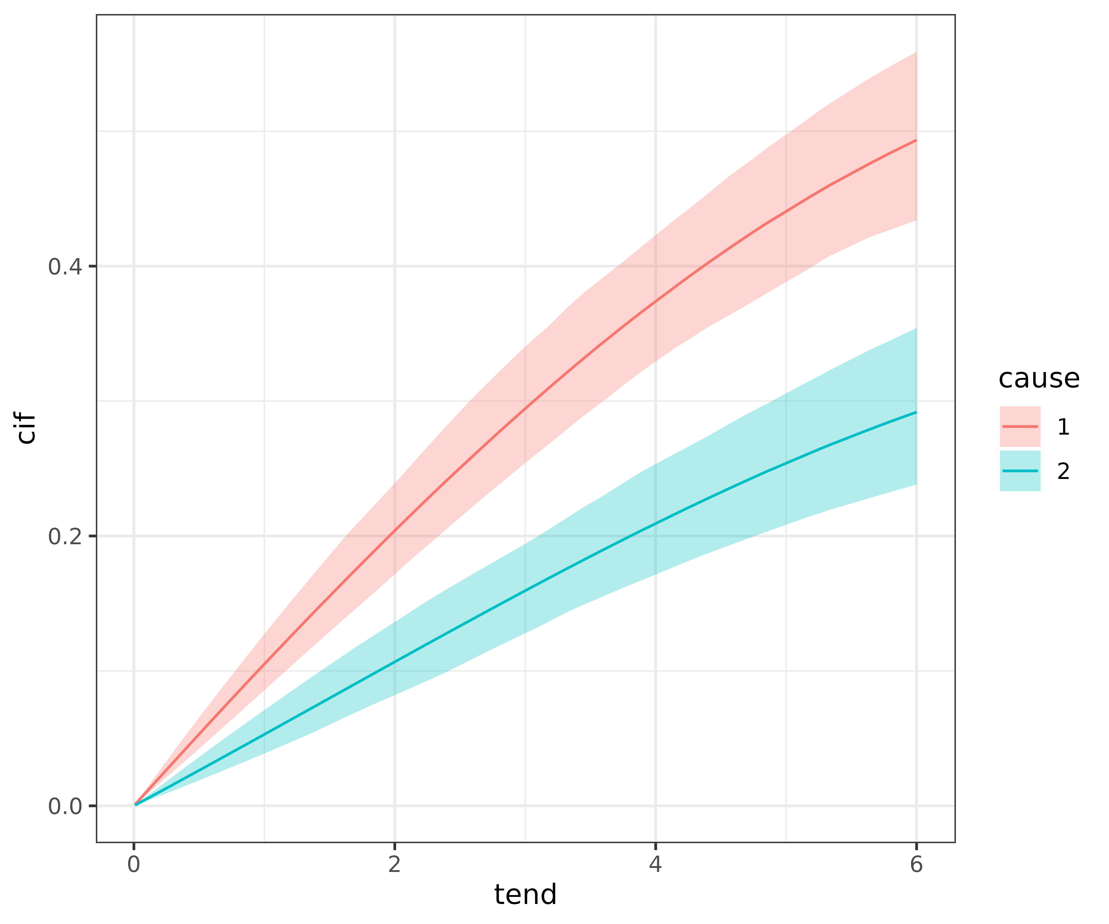

Similar to other applications of add_* functions, we can additionally group by other covariate values:

ndf <- ped_stacked %>%
  make_newdata(tend = unique(tend), cause = unique(cause), sex = unique(sex))
ndf <- ndf %>%
  group_by(cause, sex) %>%
  add_cif(pam_csh_shared)

The estimated CIFs can then be compared w.r.t. to cause for each category of sex:

ggplot(ndf, aes(x = tend, y = cif)) +
  geom_line(aes(col = cause)) +
  geom_ribbon(
    aes(ymin = cif_lower, ymax = cif_upper, fill = cause),
    alpha = .3) +
  facet_wrap(~sex, labeller = label_both)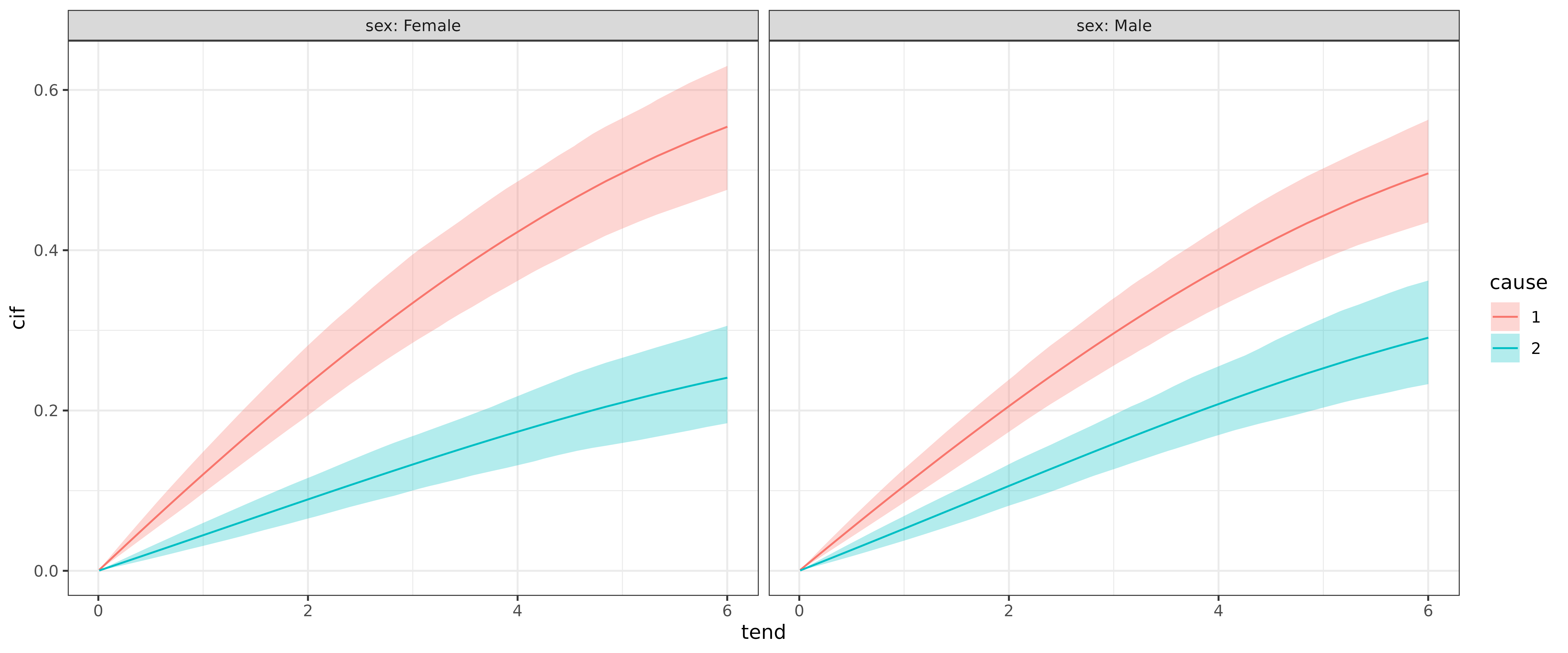

or w.r.t. to sex for each cause:

ggplot(ndf, aes(x = tend, y = cif)) +
  geom_line(aes(col = sex)) +
  geom_ribbon(
    aes(ymin = cif_lower, ymax = cif_upper, fill = sex),
    alpha = .3) +
  facet_wrap(~cause, labeller = label_both)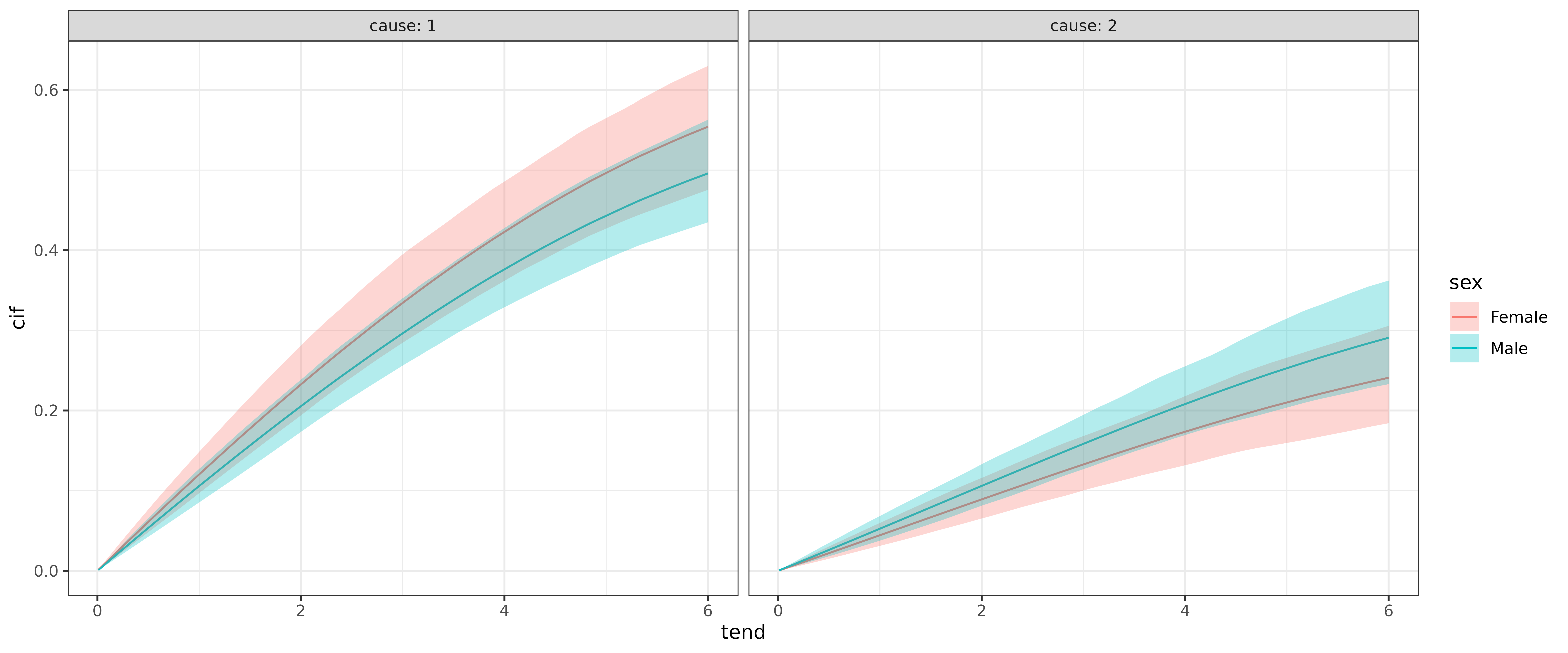

Custom time points

In the examples above, we used all unique interval grid points as time points at which the CIF was calculated. However, it is also possible to evaluate the CIF at custom time points; the calculations remain exact via the closed-form formula (1) with the truncated last interval $\Delta_{j(t)} = t - \kappa_{j(t)-1}$ (the time grid used for calculation is the same as before and expanded internally if necessary).

custom_times <- c(1, 2.5, 4)

ndf_custom <- ped_stacked %>%
  make_newdata(tend = custom_times, cause = unique(cause)) %>%
  group_by(cause) %>%
  add_cif(pam_csh_shared)

ndf_custom %>%
  select(tend, cause, cif, cif_lower, cif_upper) %>%
  arrange(tend, cause)

## # A tibble: 6 × 5
## # Groups:   cause [2]
##    tend cause    cif cif_lower cif_upper
##   <dbl> <fct>  <dbl>     <dbl>     <dbl>
## 1   1   1     0.106     0.0852    0.129 
## 2   1   2     0.0528    0.0388    0.0702
## 3   2.5 1     0.253     0.215     0.295 
## 4   2.5 2     0.133     0.105     0.171 
## 5   4   1     0.380     0.327     0.434 
## 6   4   2     0.209     0.170     0.259

Note that the confidence intervals are stochastic, as they are obtained from a Monte Carlo simulation of the model coefficients.

Andreas Bender

2026-05-04

`fourD` Data

Data transformation

Cause specific hazards model without shared effects

Cause specific hazards with shared effects

Cumulative Incidence Function (CIF)

Custom time points

Competing Risks

Andreas Bender

2026-05-04

fourD Data

Data transformation

Cause specific hazards model without shared effects

Cause specific hazards with shared effects

Cumulative Incidence Function (CIF)

Custom time points

`fourD` Data