Left Truncation

In this vignette we briefly illustrate how to fit PAMMs for left-truncated data. As an example we use the data already discussed in the left-truncation section of the data transformation vignette.

We first we load some libraries as well as the data.

library(eha)
library(pammtools)
library(ggplot2)
theme_set(theme_bw())
data(infants, package = "eha")
head(infants)

##   stratum enter exit event mother age  sex      parish   civst    ses year
## 1       1    55  365     0   dead  26  boy Nedertornea married farmer 1877
## 2       1    55  365     0  alive  26  boy Nedertornea married farmer 1870
## 3       1    55  365     0  alive  26  boy Nedertornea married farmer 1882
## 4       2    13   76     1   dead  23 girl Nedertornea married  other 1847
## 5       2    13  365     0  alive  23 girl Nedertornea married  other 1847
## 6       2    13  365     0  alive  23 girl Nedertornea married  other 1848

The header shows that we have information on entry (enter) and exit (exit) times into the riskset. Survival is indicated by the event variable. The variable of interest is mother, i.e., whether mother was alive or dead. For each child who’s mother died, 2 children of the same age and same values for the other covariates were included into the study who’s mother was still alive at inclusion age. The maximum follow up was 365 days.

As a proof of concept we show that we can recreate the effects found by the Cox model for left truncated data as implemented in eha::coxreg:

# fit cox model for left-truncated data
fit <- coxreg(
  formula = Surv(enter, exit, event) ~  mother,
  data = infants)
# fit pam to left-truncated data
infants_ped <- infants %>% as_ped(Surv(enter, exit, event)~.)
pam <- pamm(
  formula = ped_status ~ s(tend)+ mother,
  trafo_args = list(formula = Surv(enter, exit, event)~.),
  data = infants)
# compare coefficients
cbind(coef(pam)[2], coef(fit))

##               [,1]    [,2]
## motherdead 1.68071 1.69185

The coefficients of the mother variable are very similar and indicate that children with diseased mother’s are about 5.37 times as likely to die within one year after birth.

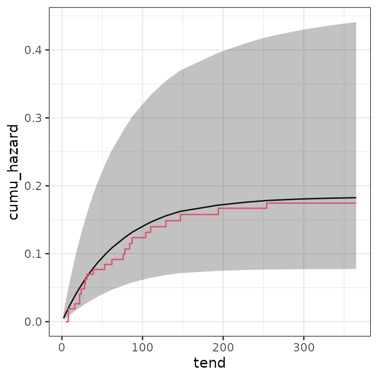
## compare (baseline) cumulative hazard probabilities
base <- survival::basehaz(fit)
ndf <- make_newdata(infants_ped, tend = unique(tend), mother = c("alive")) %>%
  add_cumu_hazard(pam)
ggplot(ndf, aes(x = tend, y = cumu_hazard)) +
  geom_line() +
  geom_ribbon(aes(ymin = cumu_lower, ymax = cumu_upper), alpha = .3) +
  geom_step(data = base, aes(x = time, y = hazard), col = 2)

2024-02-26