Recurrent Events

Introduction

We illustrate application of PAMMs in the analysis of the effect of HIV exposure on the time to staphylococcus aureaus infection in children, with possible recurrences. The children are anonymized and random ids were generated. The following packages are used in this analysis:

library(mgcv)
library(pammtools)
library(dplyr) #data wrangling
library(ggplot2) #visualization
theme_set(theme_bw())

Time until staphylococcus aureaus infection in children

The data set (staph), is contained within the pammtools package and includes 374 observations from 137 children (from the Drakenstein child health study) with a maximum of 6 recurrences. The staph data is in longitudinal format reflecting the recurrences for children over different rows. Here

t.start and t.stop indicate the entry and exit time into the risk set for the respective recurrences
event indicates whether the \(k\)-th recurrence was observed (1 = yes, 0 = censored for the \(k\)-th recurrence)
enum is the event number \(k\)
HIVexposure indicates whether the mother of the child was HIV positive (1 = yes, 0 = no)

data("staph")
head(staph)

## # A tibble: 6 × 6
##   id    t.start t.stop event  enum   hiv
##   <fct>   <dbl>  <dbl> <dbl> <dbl> <dbl>
## 1 1           0     16     1     1     0
## 2 1          16    324     1     2     0
## 3 1         324    365     0     3     0
## 4 2           0     59     1     1     1
## 5 2          59    157     1     2     1
## 6 2         157    227     1     3     1

The data for the first two children are

staph %>% filter(id %in% c("1", "2"))

## # A tibble: 7 × 6
##   id    t.start t.stop event  enum   hiv
##   <fct>   <dbl>  <dbl> <dbl> <dbl> <dbl>
## 1 1           0     16     1     1     0
## 2 1          16    324     1     2     0
## 3 1         324    365     0     3     0
## 4 2           0     59     1     1     1
## 5 2          59    157     1     2     1
## 6 2         157    227     1     3     1
## 7 2         227    368     0     4     1

Transformation to PED format

In order to apply PAMMs to recurrent events, we first transform the data to the piece-wise exponential data (PED) format (see here for details). We use the as_ped() function in pammtools. For the data transformation in the recurrent events context, we first need to decide whether analysis should be performed on the calendar- or gap-time scale. This is controlled by the timescale argument (see below). For these data, we use the gap-time.

The individual inputs for the data transformation are given as follows:

formula: specifies the Surv object on the left hand side which contains information about the risk set entry and exit times as well as the event indicator; and the variables that should be retained in the data set after data transformation. Note that the variables id and enum will be retained in the data without specification.
id: specifies the variable in the data set the indicates individual subjects
data: the data to be transformed
transition: the variable that indicates transitions from one state to another (here state transitions are transitions from event number \(k-1\) to \(k\))
timescale: the time scale of the output data (defaults to gap time)
max_time: The maximum time considered. All observations with \(t>max\_time\) will be set to max_time and their event indicator set to \(0\). Here we restrict the follow-up to 366 days, as it marks one year under observation and few children were under observation beyond that time.
cut: This argument is unspecified here, but could be used to control the time points at which the follow-up is partitioned. If unspecified, all unique event times are used as cut points.

ped <- as_ped(
  formula     = Surv(t.start,t.stop,event) ~ hiv,
  id          = "id",
  data        = staph,
  transition  = "enum",
  timescale   = "gap",
  max_time    = 366)

The resulting data for the first two infants is indicated below (we show the first and last observation of each infant for each event number they were at risk):

ped %>%
  filter(id %in% c("1", "2")) %>%
  group_by(id, enum) %>%
  slice(1, n())

## # A tibble: 14 × 8
## # Groups:   id, enum [7]
##    id    tstart  tend interval  offset ped_status   hiv  enum
##  * <fct>  <dbl> <dbl> <fct>      <dbl>      <dbl> <dbl> <dbl>
##  1 1          0     1 (0,1]      0              0     0     1
##  2 1         15    16 (15,16]    0              1     0     1
##  3 1          0     1 (0,1]      0              0     0     2
##  4 1        295   308 (295,308]  2.56           1     0     2
##  5 1          0     1 (0,1]      0              0     0     3
##  6 1         40    41 (40,41]    0              0     0     3
##  7 2          0     1 (0,1]      0              0     1     1
##  8 2         57    59 (57,59]    0.693          1     1     1
##  9 2          0     1 (0,1]      0              0     1     2
## 10 2         97    98 (97,98]    0              1     1     2
## 11 2          0     1 (0,1]      0              0     1     3
## 12 2         69    70 (69,70]    0              1     1     3
## 13 2          0     1 (0,1]      0              0     1     4
## 14 2        140   141 (140,141]  0              0     1     4

Baseline model

Model specification

We first model the baseline hazards over time. Biologically, the infection incidence in gap time may be different for the first event compared with the recurrences. However, estimation of the baseline hazard for each of the event numbers is not useful/feasible since only a few subjects experienced 3 or more events. Therefore, we will create a new variable to indicate whether the event a child is at risk for is the first event or a recurrence. Note, however, that we do this after PED data transformation and use the full information to create the PED data. We only use enum_strata for stratification when estimating the baseline hazard.

ped <- ped %>%
  mutate(enum_strata = as.factor(ifelse(enum > 1,"recurrent","first")))

Using this data, we fit the following model

\[ \lambda(t,k|z_i) = \exp(\beta_{0k} + f_{0,k}(t) + z_i), \]

where \(z_i\sim N(0, \sigma_z^2)\) are Gaussian, child specific random effects that account for child-specific frailty and \(\beta_{0k}\) and \(f_{0k}\) are the constant (intercept) and non-linear parts of the log-baseline hazard of the \(k\)-th event. Given the data transformation, this is equivalent to fitting a stratified PAM (see here for details), where stratification is done w.r.t. to enum_strata.

Fitting the model

Details on the model specification in R are given below. Note that we use the pamm function to fit the model, which is a wrapper to mgcv::gam or mgcv::bam, but direct modeling of the data using any suitable package/function would also be possible. The other arguments are passed to the respective fitting function.

In the formula argument,

s(tend, by = enum_strata) indicates the non-linear smooth functions, estimated via penalized splines (with thin-plate spline basis functions). By using by=enum_strata inside s() and including enum_strata as a fixed effect in the model, we are modeling stratified smooth functions (i.e., stratified baseline hazards) for first and recurrent events respectively, and
s(id, bs = "re") indicates a random effect (frailty) for each child.

pamm0 <- pamm(
  formula  = ped_status ~ enum_strata + s(tend, by = enum_strata) + s(id, bs = "re"),
  data     = ped,
  engine   = "bam",
  method   = "fREML",
  discrete = TRUE)

As usual for mgcv objects, the resulting model summary output shown below is separated into two parts, one for the “parametric coefficients” and one for the “smooth terms”. In case of smooth terms, the estimated degrees of freedom (edf) gives us an idea of how “wiggly” the respective smooth functions are, and the p-values test whether overall these are different from a flat line (Wood 2013). For the random effects terms, we report their estimated variances (gam.vcomp) and p-values (summary output). From the output, we see that the random effects are statistically insignificant \((p=0.249)\).

summary(pamm0)

## 
## Family: poisson 
## Link function: log 
## 
## Formula:
## ped_status ~ enum_strata + s(tend, by = enum_strata) + s(id, 
##     bs = "re")
## 
## Parametric coefficients:
##                      Estimate Std. Error z value Pr(>|z|)    
## (Intercept)           -4.9287     0.1213  -40.62  < 2e-16 ***
## enum_stratarecurrent  -1.0991     0.1857   -5.92 3.23e-09 ***
## ---
## Signif. codes:  0 '***' 0.001 '**' 0.01 '*' 0.05 '.' 0.1 ' ' 1
## 
## Approximate significance of smooth terms:
##                                 edf  Ref.df Chi.sq p-value    
## s(tend):enum_stratafirst      1.995   2.487  35.69 < 2e-16 ***
## s(tend):enum_stratarecurrent  6.101   7.240  33.49 3.7e-05 ***
## s(id)                        14.052 136.000  15.17   0.249    
## ---
## Signif. codes:  0 '***' 0.001 '**' 0.01 '*' 0.05 '.' 0.1 ' ' 1
## 
## R-sq.(adj) =  -0.0265   Deviance explained = -0.97%
## fREML =  18453  Scale est. = 1         n = 18889

The standard deviation of the random effects is also relatively small and can be extracted using the gam.vcomp command:

gam.vcomp(pamm0)

## 
## Standard deviations and 0.95 confidence intervals:
## 
##                                   std.dev        lower       upper
## s(tend):enum_stratafirst     0.0005741588 8.308116e-05 0.003967907
## s(tend):enum_stratarecurrent 0.0062687807 2.563565e-03 0.015329284
## s(id)                        0.2565797067 4.015591e-02 1.639438617
## 
## Rank: 3/3

The results indicate that random effects are not required in this model. We therefore omit the random effects in the following.

pam0 <- update(pamm0, .~. - s(id, bs = "re"))
summary(pam0)

## 
## Family: poisson 
## Link function: log 
## 
## Formula:
## ped_status ~ enum_strata + s(tend, by = enum_strata)
## 
## Parametric coefficients:
##                      Estimate Std. Error z value Pr(>|z|)    
## (Intercept)           -5.0624     0.1231 -41.124  < 2e-16 ***
## enum_stratarecurrent  -0.8860     0.1801  -4.919 8.71e-07 ***
## ---
## Signif. codes:  0 '***' 0.001 '**' 0.01 '*' 0.05 '.' 0.1 ' ' 1
## 
## Approximate significance of smooth terms:
##                                edf Ref.df Chi.sq  p-value    
## s(tend):enum_stratafirst     2.099  2.616  41.71  < 2e-16 ***
## s(tend):enum_stratarecurrent 6.099  7.238  33.07 3.98e-05 ***
## ---
## Signif. codes:  0 '***' 0.001 '**' 0.01 '*' 0.05 '.' 0.1 ' ' 1
## 
## R-sq.(adj) =  -0.0276   Deviance explained = -2.34%
## fREML =  18453  Scale est. = 1         n = 18889

Estimates over time and visualization

To obtain and visualize any quantity based on the fitted model, it is easiest to create a suitable data set and calculate the quantity of interest. pammtools provides the respective convenience functions.

Below we illustrate the calculation and visualization of the baseline hazard over time, where we use

make_newdata to create a data set with one row for each unique event time used when fitting the model, stratified by event stratum. make_newdata constructs a combination of the variables specified (here unique values of tend for each value of enum_strata, similar to expand.grid, and sets all other variables to mean and modus values, if applicable). It is also aware of the specific PED structure.
use the add_hazard function to augment the created data set with the predicted hazard and respective confidence intervals.

Once the data is created and augmented with the predicted hazard, we can use standard visualization function to create the graphics:

newdata <- ped %>%
  make_newdata(
    tend = unique(tend),
    enum_strata = unique(enum_strata)) %>%
  add_hazard(pamm0, type = "response")

ggplot(newdata, aes(x = tend/(365.25/12), y = hazard*365.25)) +
  geom_line() +
  geom_ribbon(aes(ymin  = ci_lower*365.25, ymax = ci_upper*365.25), alpha = .3) +
  ylab(expression(hat(h)(t))) + xlab("Time (months)") +
  scale_x_continuous(limits = c(0, 12.5),breaks=seq(0,12,2),expand=c(0,0)) +
  facet_wrap(~enum_strata)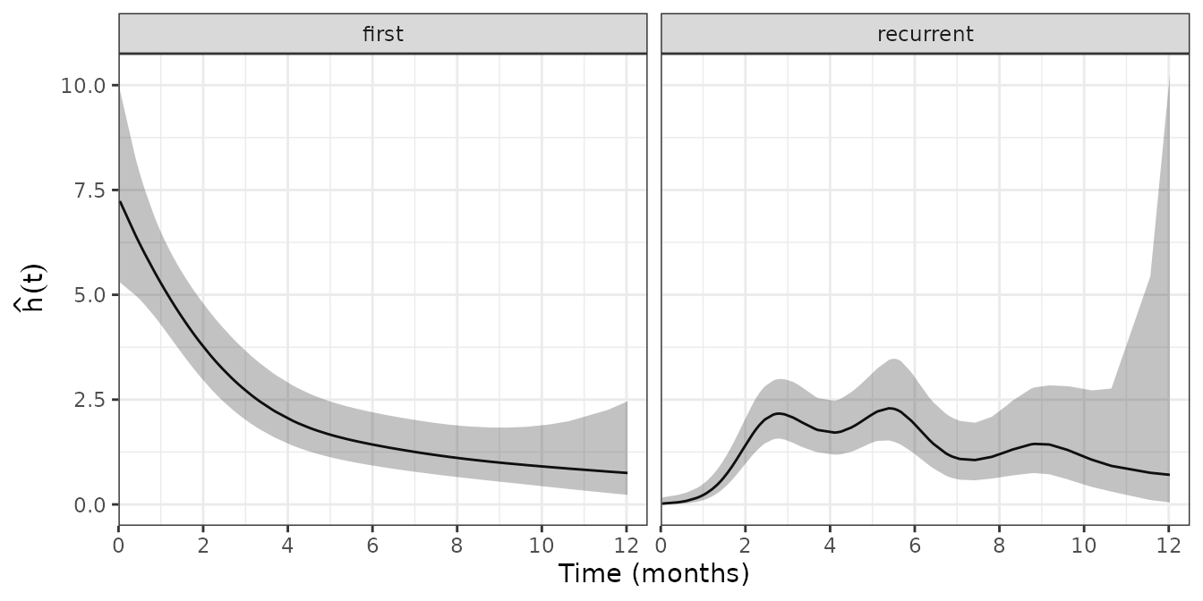

We can see, that the hazard for the first event is high in the beginning and declines over time, as most children will have had the first infection after one year of life. Consequently, the hazard for recurrence is low in the beginning and increases over time before it flattens out after about two months.

Calculation of survival probabilities works equivalently, except that we use the add_surv_prob function instead of add_hazard. Note that calculating the survival probability involves calculating a cumulative hazard. Thus, when there is a grouping structure in the data (here the different strata), we have to group by this variable before we calculate cumulative hazards or survival probabilities. Note also, that we use geom_surv in order to force the function to start at a survival probability of 1.

newdata <-newdata %>%
  group_by(enum_strata) %>%
  add_surv_prob(pamm0)

ggplot(newdata, aes(x = tend/(365.25/12), y = surv_prob)) +
  geom_surv() +
  geom_ribbon(aes(ymin  = surv_lower, ymax = surv_upper), alpha = .3) +
  ylab(expression(hat(S)(t))) + xlab("Time (months)") +
  scale_x_continuous(limits = c(0, 12.1)) +
  facet_wrap(~enum_strata)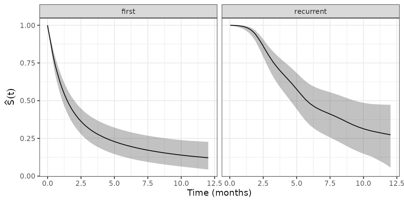

## Warning: Unknown or uninitialised column: `linewidth`.

## Warning: Unknown or uninitialised column: `size`.

Modeling the effects of HIV assuming proportional hazards

The HIV exposure variable indicates whether children were HIV exposed and uninfected (HEU) by being born to HIV positive mothers or HIV uninfected (HU). We will fit this model in the PAMM framework to evaluate the effect of HIV exposure while assuming proportional hazards. This means that the effects of HIV shift the log-hazard by some constant over time. We fit two models. In the first model, we assume that the hazard ratio is the same for first and recurrent infections. In the second model, we allow different hazard ratios for first and recurrent infections, but we still assume both these hazard ratios are proportional over time.

Model 1

pam1 <- pamm(
  formula  = ped_status ~ enum_strata + s(tend, by = enum_strata) + hiv,
  data     = ped,
  engine   = "bam",
  method   = "fREML",
  discrete = TRUE)

summary(pam1)

## 
## Family: poisson 
## Link function: log 
## 
## Formula:
## ped_status ~ enum_strata + s(tend, by = enum_strata) + hiv
## 
## Parametric coefficients:
##                      Estimate Std. Error z value Pr(>|z|)    
## (Intercept)           -5.1351     0.1303 -39.416  < 2e-16 ***
## enum_stratarecurrent  -0.8779     0.1801  -4.874 1.09e-06 ***
## hiv                    0.2681     0.1434   1.870   0.0615 .  
## ---
## Signif. codes:  0 '***' 0.001 '**' 0.01 '*' 0.05 '.' 0.1 ' ' 1
## 
## Approximate significance of smooth terms:
##                                edf Ref.df Chi.sq  p-value    
## s(tend):enum_stratafirst     2.121  2.643  41.78  < 2e-16 ***
## s(tend):enum_stratarecurrent 6.084  7.224  33.22 3.71e-05 ***
## ---
## Signif. codes:  0 '***' 0.001 '**' 0.01 '*' 0.05 '.' 0.1 ' ' 1
## 
## R-sq.(adj) =  -0.0279   Deviance explained = -2.18%
## fREML =  18453  Scale est. = 1         n = 18889

We can see that estimated effect of HIV exposure in terms of the hazard ratio is \(HR=\exp(0.2681)=1.31\;(p=0.062)\).

Model 2

pam2 <- pamm(
  formula  = ped_status ~ enum_strata + s(tend, by = enum_strata) + hiv:enum_strata,
  data     = ped,
  engine   = "bam",
  method   = "fREML",
  discrete = TRUE)

summary(pam2)

## 
## Family: poisson 
## Link function: log 
## 
## Formula:
## ped_status ~ enum_strata + s(tend, by = enum_strata) + hiv:enum_strata
## 
## Parametric coefficients:
##                          Estimate Std. Error z value Pr(>|z|)    
## (Intercept)              -5.05753    0.13330 -37.940  < 2e-16 ***
## enum_stratarecurrent     -1.03583    0.19753  -5.244 1.57e-07 ***
## enum_stratafirst:hiv     -0.02007    0.21300  -0.094  0.92493    
## enum_stratarecurrent:hiv  0.54272    0.19553   2.776  0.00551 ** 
## ---
## Signif. codes:  0 '***' 0.001 '**' 0.01 '*' 0.05 '.' 0.1 ' ' 1
## 
## Approximate significance of smooth terms:
##                                edf Ref.df Chi.sq  p-value    
## s(tend):enum_stratafirst     2.098  2.615  41.71  < 2e-16 ***
## s(tend):enum_stratarecurrent 6.067  7.208  33.42 3.24e-05 ***
## ---
## Signif. codes:  0 '***' 0.001 '**' 0.01 '*' 0.05 '.' 0.1 ' ' 1
## 
## R-sq.(adj) =  -0.0274   Deviance explained = -2.01%
## fREML =  18451  Scale est. = 1         n = 18889

We can see that estimated effect of HIV exposure in terms of the hazard ratio is \(HR=\exp(-0.0201)=0.98\;(p=0.925)\) for the first infection and \(HR=\exp(0.5427)=1.72\;(p=0.006)\) for recurrent infections.

References

Wood, Simon N. 2013. “On p-Values for Smooth Components of an Extended Generalized Additive Model.” Biometrika 100 (1): 221–28. https://doi.org/10.1093/biomet/ass048.

Jordache Ramjith, Andreas Bender, Kit C.B. Roes & Marianne A. Jonker

2024-02-26