library(ggplot2)
theme_set(theme_bw())
library(dplyr)
library(survival)
library(mgcv)
library(pammtools)
Set1 <- RColorBrewer::brewer.pal(9, "Set1")
Here we briefly demonstrate how to fit and visualize a simple
baseline model using the pammtools
package. We illustrate the procedure using a subset of the
tumor data from the pammtools
package:
## # A tibble: 6 × 9
##    days status charlson_score   age sex    transfusion complications metastases
##   <dbl>  <int>          <int> <int> <fct>  <fct>       <fct>         <fct>
## 1   579      0              2    58 female yes         no            yes
## 2  1192      0              2    52 male   no          yes           yes
## 3   308      1              2    74 female yes         no            yes
## 4    33      1              2    57 male   yes         yes           yes
## 5   397      1              2    30 female yes         no            yes
## 6  1219      0              2    66 female yes         no            yes
## # ℹ 1 more variable: resection <fct>
tumor <- tumor[1:200,]The below graph depicts the estimated cumulative hazard using the Nelson-Aalen estimator:
base_df <- basehaz(coxph(Surv(days, status)~1, data = tumor)) %>%
  rename(nelson_aalen = hazard)
ggplot(base_df, aes(x = time, y = nelson_aalen)) +
  geom_stephazard() +
  ylab(expression(hat(Lambda)(t))) + xlab("t") +
  ggtitle("Nelson-Aalen estimate of the cumulative hazard")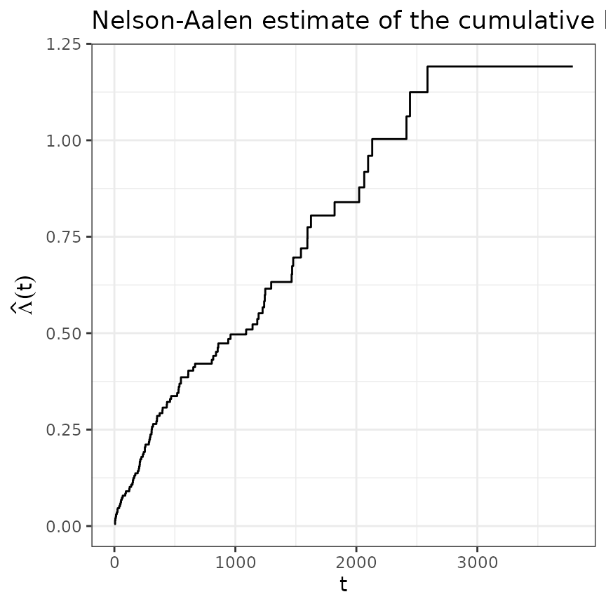
Data transformation
To fit a PAM, we first we need to bring the data in a suitable format (see vignette on data transformation).
# Use unique event times as interval break points
ped <- tumor %>% as_ped(Surv(days, status)~., id = "id")
head(ped[, 1:10])
## id tstart tend interval offset ped_status charlson_score age sex
## 1 1 0 5 (0,5] 1.6094379 0 2 58 female
## 2 1 5 8 (5,8] 1.0986123 0 2 58 female
## 3 1 8 10 (8,10] 0.6931472 0 2 58 female
## 4 1 10 14 (10,14] 1.3862944 0 2 58 female
## 5 1 14 20 (14,20] 1.7917595 0 2 58 female
## 6 1 20 26 (20,26] 1.7917595 0 2 58 female
## transfusion
## 1 yes
## 2 yes
## 3 yes
## 4 yes
## 5 yes
## 6 yesPAMs
PAMs estimate the baseline log-hazard rate semi-parametrically as a
smooth, non-linear function evaluated at the end-points
tend of the intervals defined for our model.
Note that the estimated log-hazard value at time-points
tend gives the value of the log-hazard rate for the
entire previous interval as PAMs estimate hazard rates
that are constant in each interval.
Estimating the log hazard rate as a smooth function evaluated at
tend - instead of using an unpenalized estimator without
such a smoothness assumption - ensures that the hazard rate does not
change too rapidly from interval to interval unless there is sufficient
evidence for such changes in the data.
##
## Family: poisson
## Link function: log
##
## Formula:
## ped_status ~ s(tend)
##
## Parametric coefficients:
##             Estimate Std. Error z value Pr(>|z|)
## (Intercept)  -7.4044     0.1115   -66.4   <2e-16 ***
## ---
## Signif. codes:  0 '***' 0.001 '**' 0.01 '*' 0.05 '.' 0.1 ' ' 1
##
## Approximate significance of smooth terms:
##           edf Ref.df Chi.sq p-value
## s(tend) 2.188   2.72  12.37 0.00703 **
## ---
## Signif. codes:  0 '***' 0.001 '**' 0.01 '*' 0.05 '.' 0.1 ' ' 1
##
## R-sq.(adj) =  -0.00673   Deviance explained = 1.34%
## UBRE = -0.91507  Scale est. = 1         n = 11619
Graphical comparison
In the figure below we compare the previous baseline estimates of the Cox model with the PAM estimates.
Expand here for R-Code
# Create new data set with one row per unique interval
# and add information about the cumulative hazard estimate
int_df <- make_newdata(ped, tend = unique(tend)) %>%
  add_cumu_hazard(pam)

gg_baseline <- ggplot(int_df, aes(x = tend)) +
  geom_line(aes(y = cumu_hazard, col = "PAM")) +
  geom_stephazard(data = base_df, aes(x=time, y = nelson_aalen, col = "Nelson-Aalen")) +
  scale_color_manual(
    name   = "Method",
    values = c("PAM" = "black", "Nelson-Aalen" = Set1[1])) +
  theme(legend.position = "bottom") +
  ylab(expression(hat(Lambda)(t))) + xlab("t") +
  ggtitle(paste0("Comparison of cumulative hazards estimated by\n",
    "Cox-PH (Nelson-Aalen) vs. PAM"))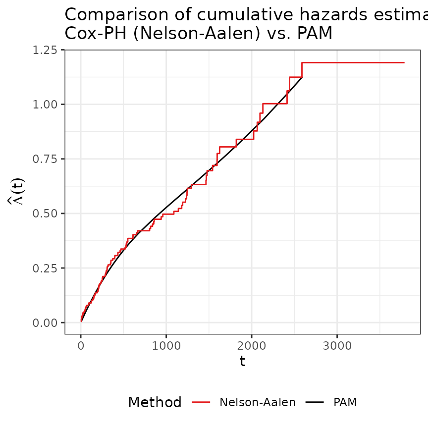
Both models are in good agreement.