Multi-State Modelling

Johannes Piller

2026-05-26

Introduction

In this vignette, we show examples of how to estimate and visualize transition probabilities for multi-state data. To validate that the PAMM baseline hazards are correctly specified, we compare the cumulative hazards transition probabilities, and their simulated confidence intervals estimated by pammtools against those from the Aalen-Johannsen estimator as implemented in mstate. Since we fit a baseline model stratified by treatment effect without additional covariates, both approaches should yield identical results up to numerical approximation from the piecewise-constant hazard assumption in PAMMs.

Example multi-state analysis: Time to abnormal prothrombin levels in liver cirrhosis using the prothr data

For illustration, we use the prothr data set from the mstate package. - 488 liver cirrhosis patients - endpoints: status = 0/1 for censoring, event - events of interest: status = 1 and to = 2/3 for abnormal prothrombin level (patient can transition between normal and abnormal prothrombin level back and forth), death, tstart, tend as time-to-event - variable of interest treat: A patient’s treatment (Placebo, Prednisone)

R-Code Setup

library(survival)
library(mgcv)
library(ggplot2)
library(pammtools)
library(purrr)
library(mstate)
library(checkmate)
library(dplyr)

theme_set(theme_bw())

data(prothr, package = "mstate")

id	from	to	trans	Tstart	Tstop	status	treat
46	1	2	1	0	415	1	Prednisone
46	1	3	2	0	415	0	Prednisone
46	2	1	3	415	417	0	Prednisone
46	2	3	4	415	417	1	Prednisone

In general, one has to follow three steps to derive transition probabilities from multi-state survival data. - First, we need to transform the survival data prothr into piecewise exponential data. - Second, we need to estimate the log hazard structure using PAM objects. - Third, we need to post-process the data to include all relevant objects of interest in our data set.

Data transformation: From raw prothr data to piecewise exponential data

The data transformation required to fit PAMMs to multi-state data extends the standard single-event piecewise exponential data (PED) transformation (see the data transformation vignette for details) to each transition type. The follow-up of each subject is split at all observed transition times across the entire dataset, and a row is added for every interval-transition combination the subject is at risk for. Two key differences arise compared to the single-event case: first, delayed entry into the risk set is handled automatically, since subjects are only at risk for transitions out of a state after they have entered it; second, competing events are treated as censoring for all other transitions within the same interval. The result is a stacked long-format dataset with one row per subject, interval, and transition, which can be passed directly to a Poisson regression model. In pammtools, this transformation is handled by as_ped() with the additional transition argument specifying the column that identifies the transition type.

data("prothr", package = "mstate")
prothr <- prothr |> 
  mutate(transition = as.factor(paste0(from, "->", to))
         , treat = as.factor(treat)) |>
  rename(tstart = Tstart, tstop = Tstop) |>
  filter(tstart != tstop) |>
  select(-trans)

ped <- as_ped(
  data       = prothr,
  formula    = Surv(tstart, tstop, status)~ .,
  transition = "transition",
  id         = "id",
  timescale  = "calendar",
  tdc_specials="concurrent"
)

Transformed PED for id == 46

ped |> filter(id == 46) |> knitr::kable()

id	tstart	tend	interval	offset	ped_status	from	to	treat	transition
46	0	4	(0,4]	1.3862944	0	1	2	Prednisone	1->2
46	4	5	(4,5]	0.0000000	0	1	2	Prednisone	1->2
46	5	13	(5,13]	2.0794415	0	1	2	Prednisone	1->2
46	13	16	(13,16]	1.0986123	0	1	2	Prednisone	1->2
46	16	21	(16,21]	1.6094379	0	1	2	Prednisone	1->2
46	21	22	(21,22]	0.0000000	0	1	2	Prednisone	1->2
46	22	23	(22,23]	0.0000000	0	1	2	Prednisone	1->2
46	23	24	(23,24]	0.0000000	0	1	2	Prednisone	1->2
46	24	25	(24,25]	0.0000000	0	1	2	Prednisone	1->2
46	25	27	(25,27]	0.6931472	0	1	2	Prednisone	1->2
46	27	29	(27,29]	0.6931472	0	1	2	Prednisone	1->2
46	29	30	(29,30]	0.0000000	0	1	2	Prednisone	1->2
46	30	31	(30,31]	0.0000000	0	1	2	Prednisone	1->2
46	31	32	(31,32]	0.0000000	0	1	2	Prednisone	1->2
46	32	33	(32,33]	0.0000000	0	1	2	Prednisone	1->2
46	33	34	(33,34]	0.0000000	0	1	2	Prednisone	1->2
46	34	35	(34,35]	0.0000000	0	1	2	Prednisone	1->2
46	35	36	(35,36]	0.0000000	0	1	2	Prednisone	1->2
46	36	37	(36,37]	0.0000000	0	1	2	Prednisone	1->2
46	37	39	(37,39]	0.6931472	0	1	2	Prednisone	1->2
46	39	40	(39,40]	0.0000000	0	1	2	Prednisone	1->2
46	40	41	(40,41]	0.0000000	0	1	2	Prednisone	1->2
46	41	43	(41,43]	0.6931472	0	1	2	Prednisone	1->2
46	43	45	(43,45]	0.6931472	0	1	2	Prednisone	1->2
46	45	48	(45,48]	1.0986123	0	1	2	Prednisone	1->2
46	48	50	(48,50]	0.6931472	0	1	2	Prednisone	1->2
46	50	53	(50,53]	1.0986123	0	1	2	Prednisone	1->2
46	53	54	(53,54]	0.0000000	0	1	2	Prednisone	1->2
46	54	58	(54,58]	1.3862944	0	1	2	Prednisone	1->2
46	58	59	(58,59]	0.0000000	0	1	2	Prednisone	1->2
46	59	63	(59,63]	1.3862944	0	1	2	Prednisone	1->2
46	63	64	(63,64]	0.0000000	0	1	2	Prednisone	1->2
46	64	66	(64,66]	0.6931472	0	1	2	Prednisone	1->2
46	66	67	(66,67]	0.0000000	0	1	2	Prednisone	1->2
46	67	70	(67,70]	1.0986123	0	1	2	Prednisone	1->2
46	70	71	(70,71]	0.0000000	0	1	2	Prednisone	1->2
46	71	72	(71,72]	0.0000000	0	1	2	Prednisone	1->2
46	72	73	(72,73]	0.0000000	0	1	2	Prednisone	1->2
46	73	74	(73,74]	0.0000000	0	1	2	Prednisone	1->2
46	74	76	(74,76]	0.6931472	0	1	2	Prednisone	1->2
46	76	77	(76,77]	0.0000000	0	1	2	Prednisone	1->2
46	77	78	(77,78]	0.0000000	0	1	2	Prednisone	1->2
46	78	80	(78,80]	0.6931472	0	1	2	Prednisone	1->2
46	80	82	(80,82]	0.6931472	0	1	2	Prednisone	1->2
46	82	83	(82,83]	0.0000000	0	1	2	Prednisone	1->2
46	83	84	(83,84]	0.0000000	0	1	2	Prednisone	1->2
46	84	85	(84,85]	0.0000000	0	1	2	Prednisone	1->2
46	85	86	(85,86]	0.0000000	0	1	2	Prednisone	1->2
46	86	87	(86,87]	0.0000000	0	1	2	Prednisone	1->2
46	87	88	(87,88]	0.0000000	0	1	2	Prednisone	1->2
46	88	89	(88,89]	0.0000000	0	1	2	Prednisone	1->2
46	89	90	(89,90]	0.0000000	0	1	2	Prednisone	1->2
46	90	91	(90,91]	0.0000000	0	1	2	Prednisone	1->2
46	91	92	(91,92]	0.0000000	0	1	2	Prednisone	1->2
46	92	93	(92,93]	0.0000000	0	1	2	Prednisone	1->2
46	93	94	(93,94]	0.0000000	0	1	2	Prednisone	1->2
46	94	95	(94,95]	0.0000000	0	1	2	Prednisone	1->2
46	95	96	(95,96]	0.0000000	0	1	2	Prednisone	1->2
46	96	97	(96,97]	0.0000000	0	1	2	Prednisone	1->2
46	97	98	(97,98]	0.0000000	0	1	2	Prednisone	1->2
46	98	99	(98,99]	0.0000000	0	1	2	Prednisone	1->2
46	99	100	(99,100]	0.0000000	0	1	2	Prednisone	1->2
46	100	101	(100,101]	0.0000000	0	1	2	Prednisone	1->2
46	101	103	(101,103]	0.6931472	0	1	2	Prednisone	1->2
46	103	104	(103,104]	0.0000000	0	1	2	Prednisone	1->2
46	104	105	(104,105]	0.0000000	0	1	2	Prednisone	1->2
46	105	108	(105,108]	1.0986123	0	1	2	Prednisone	1->2
46	108	109	(108,109]	0.0000000	0	1	2	Prednisone	1->2
46	109	110	(109,110]	0.0000000	0	1	2	Prednisone	1->2
46	110	111	(110,111]	0.0000000	0	1	2	Prednisone	1->2
46	111	112	(111,112]	0.0000000	0	1	2	Prednisone	1->2
46	112	113	(112,113]	0.0000000	0	1	2	Prednisone	1->2
46	113	114	(113,114]	0.0000000	0	1	2	Prednisone	1->2
46	114	115	(114,115]	0.0000000	0	1	2	Prednisone	1->2
46	115	116	(115,116]	0.0000000	0	1	2	Prednisone	1->2
46	116	117	(116,117]	0.0000000	0	1	2	Prednisone	1->2
46	117	118	(117,118]	0.0000000	0	1	2	Prednisone	1->2
46	118	119	(118,119]	0.0000000	0	1	2	Prednisone	1->2
46	119	120	(119,120]	0.0000000	0	1	2	Prednisone	1->2
46	120	121	(120,121]	0.0000000	0	1	2	Prednisone	1->2
46	121	122	(121,122]	0.0000000	0	1	2	Prednisone	1->2
46	122	123	(122,123]	0.0000000	0	1	2	Prednisone	1->2
46	123	124	(123,124]	0.0000000	0	1	2	Prednisone	1->2
46	124	126	(124,126]	0.6931472	0	1	2	Prednisone	1->2
46	126	127	(126,127]	0.0000000	0	1	2	Prednisone	1->2
46	127	128	(127,128]	0.0000000	0	1	2	Prednisone	1->2
46	128	129	(128,129]	0.0000000	0	1	2	Prednisone	1->2
46	129	132	(129,132]	1.0986123	0	1	2	Prednisone	1->2
46	132	136	(132,136]	1.3862944	0	1	2	Prednisone	1->2
46	136	137	(136,137]	0.0000000	0	1	2	Prednisone	1->2
46	137	138	(137,138]	0.0000000	0	1	2	Prednisone	1->2
46	138	139	(138,139]	0.0000000	0	1	2	Prednisone	1->2
46	139	140	(139,140]	0.0000000	0	1	2	Prednisone	1->2
46	140	141	(140,141]	0.0000000	0	1	2	Prednisone	1->2
46	141	142	(141,142]	0.0000000	0	1	2	Prednisone	1->2
46	142	143	(142,143]	0.0000000	0	1	2	Prednisone	1->2
46	143	147	(143,147]	1.3862944	0	1	2	Prednisone	1->2
46	147	151	(147,151]	1.3862944	0	1	2	Prednisone	1->2
46	151	152	(151,152]	0.0000000	0	1	2	Prednisone	1->2
46	152	154	(152,154]	0.6931472	0	1	2	Prednisone	1->2
46	154	155	(154,155]	0.0000000	0	1	2	Prednisone	1->2
46	155	156	(155,156]	0.0000000	0	1	2	Prednisone	1->2
46	156	160	(156,160]	1.3862944	0	1	2	Prednisone	1->2
46	160	161	(160,161]	0.0000000	0	1	2	Prednisone	1->2
46	161	163	(161,163]	0.6931472	0	1	2	Prednisone	1->2
46	163	164	(163,164]	0.0000000	0	1	2	Prednisone	1->2
46	164	166	(164,166]	0.6931472	0	1	2	Prednisone	1->2
46	166	167	(166,167]	0.0000000	0	1	2	Prednisone	1->2
46	167	168	(167,168]	0.0000000	0	1	2	Prednisone	1->2
46	168	170	(168,170]	0.6931472	0	1	2	Prednisone	1->2
46	170	173	(170,173]	1.0986123	0	1	2	Prednisone	1->2
46	173	176	(173,176]	1.0986123	0	1	2	Prednisone	1->2
46	176	177	(176,177]	0.0000000	0	1	2	Prednisone	1->2
46	177	178	(177,178]	0.0000000	0	1	2	Prednisone	1->2
46	178	180	(178,180]	0.6931472	0	1	2	Prednisone	1->2
46	180	181	(180,181]	0.0000000	0	1	2	Prednisone	1->2
46	181	182	(181,182]	0.0000000	0	1	2	Prednisone	1->2
46	182	183	(182,183]	0.0000000	0	1	2	Prednisone	1->2
46	183	184	(183,184]	0.0000000	0	1	2	Prednisone	1->2
46	184	186	(184,186]	0.6931472	0	1	2	Prednisone	1->2
46	186	187	(186,187]	0.0000000	0	1	2	Prednisone	1->2
46	187	188	(187,188]	0.0000000	0	1	2	Prednisone	1->2
46	188	189	(188,189]	0.0000000	0	1	2	Prednisone	1->2
46	189	190	(189,190]	0.0000000	0	1	2	Prednisone	1->2
46	190	191	(190,191]	0.0000000	0	1	2	Prednisone	1->2
46	191	192	(191,192]	0.0000000	0	1	2	Prednisone	1->2
46	192	193	(192,193]	0.0000000	0	1	2	Prednisone	1->2
46	193	194	(193,194]	0.0000000	0	1	2	Prednisone	1->2
46	194	195	(194,195]	0.0000000	0	1	2	Prednisone	1->2
46	195	196	(195,196]	0.0000000	0	1	2	Prednisone	1->2
46	196	197	(196,197]	0.0000000	0	1	2	Prednisone	1->2
46	197	198	(197,198]	0.0000000	0	1	2	Prednisone	1->2
46	198	201	(198,201]	1.0986123	0	1	2	Prednisone	1->2
46	201	202	(201,202]	0.0000000	0	1	2	Prednisone	1->2
46	202	203	(202,203]	0.0000000	0	1	2	Prednisone	1->2
46	203	204	(203,204]	0.0000000	0	1	2	Prednisone	1->2
46	204	205	(204,205]	0.0000000	0	1	2	Prednisone	1->2
46	205	206	(205,206]	0.0000000	0	1	2	Prednisone	1->2
46	206	207	(206,207]	0.0000000	0	1	2	Prednisone	1->2
46	207	209	(207,209]	0.6931472	0	1	2	Prednisone	1->2
46	209	210	(209,210]	0.0000000	0	1	2	Prednisone	1->2
46	210	211	(210,211]	0.0000000	0	1	2	Prednisone	1->2
46	211	212	(211,212]	0.0000000	0	1	2	Prednisone	1->2
46	212	213	(212,213]	0.0000000	0	1	2	Prednisone	1->2
46	213	214	(213,214]	0.0000000	0	1	2	Prednisone	1->2
46	214	215	(214,215]	0.0000000	0	1	2	Prednisone	1->2
46	215	216	(215,216]	0.0000000	0	1	2	Prednisone	1->2
46	216	217	(216,217]	0.0000000	0	1	2	Prednisone	1->2
46	217	218	(217,218]	0.0000000	0	1	2	Prednisone	1->2
46	218	222	(218,222]	1.3862944	0	1	2	Prednisone	1->2
46	222	223	(222,223]	0.0000000	0	1	2	Prednisone	1->2
46	223	224	(223,224]	0.0000000	0	1	2	Prednisone	1->2
46	224	225	(224,225]	0.0000000	0	1	2	Prednisone	1->2
46	225	226	(225,226]	0.0000000	0	1	2	Prednisone	1->2
46	226	229	(226,229]	1.0986123	0	1	2	Prednisone	1->2
46	229	230	(229,230]	0.0000000	0	1	2	Prednisone	1->2
46	230	231	(230,231]	0.0000000	0	1	2	Prednisone	1->2
46	231	235	(231,235]	1.3862944	0	1	2	Prednisone	1->2
46	235	238	(235,238]	1.0986123	0	1	2	Prednisone	1->2
46	238	240	(238,240]	0.6931472	0	1	2	Prednisone	1->2
46	240	245	(240,245]	1.6094379	0	1	2	Prednisone	1->2
46	245	249	(245,249]	1.3862944	0	1	2	Prednisone	1->2
46	249	251	(249,251]	0.6931472	0	1	2	Prednisone	1->2
46	251	254	(251,254]	1.0986123	0	1	2	Prednisone	1->2
46	254	256	(254,256]	0.6931472	0	1	2	Prednisone	1->2
46	256	257	(256,257]	0.0000000	0	1	2	Prednisone	1->2
46	257	261	(257,261]	1.3862944	0	1	2	Prednisone	1->2
46	261	263	(261,263]	0.6931472	0	1	2	Prednisone	1->2
46	263	266	(263,266]	1.0986123	0	1	2	Prednisone	1->2
46	266	270	(266,270]	1.3862944	0	1	2	Prednisone	1->2
46	270	271	(270,271]	0.0000000	0	1	2	Prednisone	1->2
46	271	272	(271,272]	0.0000000	0	1	2	Prednisone	1->2
46	272	273	(272,273]	0.0000000	0	1	2	Prednisone	1->2
46	273	274	(273,274]	0.0000000	0	1	2	Prednisone	1->2
46	274	276	(274,276]	0.6931472	0	1	2	Prednisone	1->2
46	276	281	(276,281]	1.6094379	0	1	2	Prednisone	1->2
46	281	283	(281,283]	0.6931472	0	1	2	Prednisone	1->2
46	283	286	(283,286]	1.0986123	0	1	2	Prednisone	1->2
46	286	290	(286,290]	1.3862944	0	1	2	Prednisone	1->2
46	290	298	(290,298]	2.0794415	0	1	2	Prednisone	1->2
46	298	301	(298,301]	1.0986123	0	1	2	Prednisone	1->2
46	301	304	(301,304]	1.0986123	0	1	2	Prednisone	1->2
46	304	308	(304,308]	1.3862944	0	1	2	Prednisone	1->2
46	308	309	(308,309]	0.0000000	0	1	2	Prednisone	1->2
46	309	312	(309,312]	1.0986123	0	1	2	Prednisone	1->2
46	312	323	(312,323]	2.3978953	0	1	2	Prednisone	1->2
46	323	325	(323,325]	0.6931472	0	1	2	Prednisone	1->2
46	325	326	(325,326]	0.0000000	0	1	2	Prednisone	1->2
46	326	329	(326,329]	1.0986123	0	1	2	Prednisone	1->2
46	329	332	(329,332]	1.0986123	0	1	2	Prednisone	1->2
46	332	336	(332,336]	1.3862944	0	1	2	Prednisone	1->2
46	336	337	(336,337]	0.0000000	0	1	2	Prednisone	1->2
46	337	339	(337,339]	0.6931472	0	1	2	Prednisone	1->2
46	339	342	(339,342]	1.0986123	0	1	2	Prednisone	1->2
46	342	346	(342,346]	1.3862944	0	1	2	Prednisone	1->2
46	346	349	(346,349]	1.0986123	0	1	2	Prednisone	1->2
46	349	350	(349,350]	0.0000000	0	1	2	Prednisone	1->2
46	350	351	(350,351]	0.0000000	0	1	2	Prednisone	1->2
46	351	352	(351,352]	0.0000000	0	1	2	Prednisone	1->2
46	352	353	(352,353]	0.0000000	0	1	2	Prednisone	1->2
46	353	354	(353,354]	0.0000000	0	1	2	Prednisone	1->2
46	354	355	(354,355]	0.0000000	0	1	2	Prednisone	1->2
46	355	357	(355,357]	0.6931472	0	1	2	Prednisone	1->2
46	357	358	(357,358]	0.0000000	0	1	2	Prednisone	1->2
46	358	359	(358,359]	0.0000000	0	1	2	Prednisone	1->2
46	359	360	(359,360]	0.0000000	0	1	2	Prednisone	1->2
46	360	361	(360,361]	0.0000000	0	1	2	Prednisone	1->2
46	361	362	(361,362]	0.0000000	0	1	2	Prednisone	1->2
46	362	363	(362,363]	0.0000000	0	1	2	Prednisone	1->2
46	363	364	(363,364]	0.0000000	0	1	2	Prednisone	1->2
46	364	365	(364,365]	0.0000000	0	1	2	Prednisone	1->2
46	365	368	(365,368]	1.0986123	0	1	2	Prednisone	1->2
46	368	369	(368,369]	0.0000000	0	1	2	Prednisone	1->2
46	369	370	(369,370]	0.0000000	0	1	2	Prednisone	1->2
46	370	371	(370,371]	0.0000000	0	1	2	Prednisone	1->2
46	371	372	(371,372]	0.0000000	0	1	2	Prednisone	1->2
46	372	373	(372,373]	0.0000000	0	1	2	Prednisone	1->2
46	373	376	(373,376]	1.0986123	0	1	2	Prednisone	1->2
46	376	377	(376,377]	0.0000000	0	1	2	Prednisone	1->2
46	377	378	(377,378]	0.0000000	0	1	2	Prednisone	1->2
46	378	381	(378,381]	1.0986123	0	1	2	Prednisone	1->2
46	381	385	(381,385]	1.3862944	0	1	2	Prednisone	1->2
46	385	386	(385,386]	0.0000000	0	1	2	Prednisone	1->2
46	386	387	(386,387]	0.0000000	0	1	2	Prednisone	1->2
46	387	390	(387,390]	1.0986123	0	1	2	Prednisone	1->2
46	390	392	(390,392]	0.6931472	0	1	2	Prednisone	1->2
46	392	394	(392,394]	0.6931472	0	1	2	Prednisone	1->2
46	394	398	(394,398]	1.3862944	0	1	2	Prednisone	1->2
46	398	399	(398,399]	0.0000000	0	1	2	Prednisone	1->2
46	399	402	(399,402]	1.0986123	0	1	2	Prednisone	1->2
46	402	403	(402,403]	0.0000000	0	1	2	Prednisone	1->2
46	403	404	(403,404]	0.0000000	0	1	2	Prednisone	1->2
46	404	405	(404,405]	0.0000000	0	1	2	Prednisone	1->2
46	405	406	(405,406]	0.0000000	0	1	2	Prednisone	1->2
46	406	407	(406,407]	0.0000000	0	1	2	Prednisone	1->2
46	407	409	(407,409]	0.6931472	0	1	2	Prednisone	1->2
46	409	411	(409,411]	0.6931472	0	1	2	Prednisone	1->2
46	411	415	(411,415]	1.3862944	1	1	2	Prednisone	1->2
46	0	4	(0,4]	1.3862944	0	1	3	Prednisone	1->3
46	4	5	(4,5]	0.0000000	0	1	3	Prednisone	1->3
46	5	13	(5,13]	2.0794415	0	1	3	Prednisone	1->3
46	13	16	(13,16]	1.0986123	0	1	3	Prednisone	1->3
46	16	21	(16,21]	1.6094379	0	1	3	Prednisone	1->3
46	21	22	(21,22]	0.0000000	0	1	3	Prednisone	1->3
46	22	23	(22,23]	0.0000000	0	1	3	Prednisone	1->3
46	23	24	(23,24]	0.0000000	0	1	3	Prednisone	1->3
46	24	25	(24,25]	0.0000000	0	1	3	Prednisone	1->3
46	25	27	(25,27]	0.6931472	0	1	3	Prednisone	1->3
46	27	29	(27,29]	0.6931472	0	1	3	Prednisone	1->3
46	29	30	(29,30]	0.0000000	0	1	3	Prednisone	1->3
46	30	31	(30,31]	0.0000000	0	1	3	Prednisone	1->3
46	31	32	(31,32]	0.0000000	0	1	3	Prednisone	1->3
46	32	33	(32,33]	0.0000000	0	1	3	Prednisone	1->3
46	33	34	(33,34]	0.0000000	0	1	3	Prednisone	1->3
46	34	35	(34,35]	0.0000000	0	1	3	Prednisone	1->3
46	35	36	(35,36]	0.0000000	0	1	3	Prednisone	1->3
46	36	37	(36,37]	0.0000000	0	1	3	Prednisone	1->3
46	37	39	(37,39]	0.6931472	0	1	3	Prednisone	1->3
46	39	40	(39,40]	0.0000000	0	1	3	Prednisone	1->3
46	40	41	(40,41]	0.0000000	0	1	3	Prednisone	1->3
46	41	43	(41,43]	0.6931472	0	1	3	Prednisone	1->3
46	43	45	(43,45]	0.6931472	0	1	3	Prednisone	1->3
46	45	48	(45,48]	1.0986123	0	1	3	Prednisone	1->3
46	48	50	(48,50]	0.6931472	0	1	3	Prednisone	1->3
46	50	53	(50,53]	1.0986123	0	1	3	Prednisone	1->3
46	53	54	(53,54]	0.0000000	0	1	3	Prednisone	1->3
46	54	58	(54,58]	1.3862944	0	1	3	Prednisone	1->3
46	58	59	(58,59]	0.0000000	0	1	3	Prednisone	1->3
46	59	63	(59,63]	1.3862944	0	1	3	Prednisone	1->3
46	63	64	(63,64]	0.0000000	0	1	3	Prednisone	1->3
46	64	66	(64,66]	0.6931472	0	1	3	Prednisone	1->3
46	66	67	(66,67]	0.0000000	0	1	3	Prednisone	1->3
46	67	70	(67,70]	1.0986123	0	1	3	Prednisone	1->3
46	70	71	(70,71]	0.0000000	0	1	3	Prednisone	1->3
46	71	72	(71,72]	0.0000000	0	1	3	Prednisone	1->3
46	72	73	(72,73]	0.0000000	0	1	3	Prednisone	1->3
46	73	74	(73,74]	0.0000000	0	1	3	Prednisone	1->3
46	74	76	(74,76]	0.6931472	0	1	3	Prednisone	1->3
46	76	77	(76,77]	0.0000000	0	1	3	Prednisone	1->3
46	77	78	(77,78]	0.0000000	0	1	3	Prednisone	1->3
46	78	80	(78,80]	0.6931472	0	1	3	Prednisone	1->3
46	80	82	(80,82]	0.6931472	0	1	3	Prednisone	1->3
46	82	83	(82,83]	0.0000000	0	1	3	Prednisone	1->3
46	83	84	(83,84]	0.0000000	0	1	3	Prednisone	1->3
46	84	85	(84,85]	0.0000000	0	1	3	Prednisone	1->3
46	85	86	(85,86]	0.0000000	0	1	3	Prednisone	1->3
46	86	87	(86,87]	0.0000000	0	1	3	Prednisone	1->3
46	87	88	(87,88]	0.0000000	0	1	3	Prednisone	1->3
46	88	89	(88,89]	0.0000000	0	1	3	Prednisone	1->3
46	89	90	(89,90]	0.0000000	0	1	3	Prednisone	1->3
46	90	91	(90,91]	0.0000000	0	1	3	Prednisone	1->3
46	91	92	(91,92]	0.0000000	0	1	3	Prednisone	1->3
46	92	93	(92,93]	0.0000000	0	1	3	Prednisone	1->3
46	93	94	(93,94]	0.0000000	0	1	3	Prednisone	1->3
46	94	95	(94,95]	0.0000000	0	1	3	Prednisone	1->3
46	95	96	(95,96]	0.0000000	0	1	3	Prednisone	1->3
46	96	97	(96,97]	0.0000000	0	1	3	Prednisone	1->3
46	97	98	(97,98]	0.0000000	0	1	3	Prednisone	1->3
46	98	99	(98,99]	0.0000000	0	1	3	Prednisone	1->3
46	99	100	(99,100]	0.0000000	0	1	3	Prednisone	1->3
46	100	101	(100,101]	0.0000000	0	1	3	Prednisone	1->3
46	101	103	(101,103]	0.6931472	0	1	3	Prednisone	1->3
46	103	104	(103,104]	0.0000000	0	1	3	Prednisone	1->3
46	104	105	(104,105]	0.0000000	0	1	3	Prednisone	1->3
46	105	108	(105,108]	1.0986123	0	1	3	Prednisone	1->3
46	108	109	(108,109]	0.0000000	0	1	3	Prednisone	1->3
46	109	110	(109,110]	0.0000000	0	1	3	Prednisone	1->3
46	110	111	(110,111]	0.0000000	0	1	3	Prednisone	1->3
46	111	112	(111,112]	0.0000000	0	1	3	Prednisone	1->3
46	112	113	(112,113]	0.0000000	0	1	3	Prednisone	1->3
46	113	114	(113,114]	0.0000000	0	1	3	Prednisone	1->3
46	114	115	(114,115]	0.0000000	0	1	3	Prednisone	1->3
46	115	116	(115,116]	0.0000000	0	1	3	Prednisone	1->3
46	116	117	(116,117]	0.0000000	0	1	3	Prednisone	1->3
46	117	118	(117,118]	0.0000000	0	1	3	Prednisone	1->3
46	118	119	(118,119]	0.0000000	0	1	3	Prednisone	1->3
46	119	120	(119,120]	0.0000000	0	1	3	Prednisone	1->3
46	120	121	(120,121]	0.0000000	0	1	3	Prednisone	1->3
46	121	122	(121,122]	0.0000000	0	1	3	Prednisone	1->3
46	122	123	(122,123]	0.0000000	0	1	3	Prednisone	1->3
46	123	124	(123,124]	0.0000000	0	1	3	Prednisone	1->3
46	124	126	(124,126]	0.6931472	0	1	3	Prednisone	1->3
46	126	127	(126,127]	0.0000000	0	1	3	Prednisone	1->3
46	127	128	(127,128]	0.0000000	0	1	3	Prednisone	1->3
46	128	129	(128,129]	0.0000000	0	1	3	Prednisone	1->3
46	129	132	(129,132]	1.0986123	0	1	3	Prednisone	1->3
46	132	136	(132,136]	1.3862944	0	1	3	Prednisone	1->3
46	136	137	(136,137]	0.0000000	0	1	3	Prednisone	1->3
46	137	138	(137,138]	0.0000000	0	1	3	Prednisone	1->3
46	138	139	(138,139]	0.0000000	0	1	3	Prednisone	1->3
46	139	140	(139,140]	0.0000000	0	1	3	Prednisone	1->3
46	140	141	(140,141]	0.0000000	0	1	3	Prednisone	1->3
46	141	142	(141,142]	0.0000000	0	1	3	Prednisone	1->3
46	142	143	(142,143]	0.0000000	0	1	3	Prednisone	1->3
46	143	147	(143,147]	1.3862944	0	1	3	Prednisone	1->3
46	147	151	(147,151]	1.3862944	0	1	3	Prednisone	1->3
46	151	152	(151,152]	0.0000000	0	1	3	Prednisone	1->3
46	152	154	(152,154]	0.6931472	0	1	3	Prednisone	1->3
46	154	155	(154,155]	0.0000000	0	1	3	Prednisone	1->3
46	155	156	(155,156]	0.0000000	0	1	3	Prednisone	1->3
46	156	160	(156,160]	1.3862944	0	1	3	Prednisone	1->3
46	160	161	(160,161]	0.0000000	0	1	3	Prednisone	1->3
46	161	163	(161,163]	0.6931472	0	1	3	Prednisone	1->3
46	163	164	(163,164]	0.0000000	0	1	3	Prednisone	1->3
46	164	166	(164,166]	0.6931472	0	1	3	Prednisone	1->3
46	166	167	(166,167]	0.0000000	0	1	3	Prednisone	1->3
46	167	168	(167,168]	0.0000000	0	1	3	Prednisone	1->3
46	168	170	(168,170]	0.6931472	0	1	3	Prednisone	1->3
46	170	173	(170,173]	1.0986123	0	1	3	Prednisone	1->3
46	173	176	(173,176]	1.0986123	0	1	3	Prednisone	1->3
46	176	177	(176,177]	0.0000000	0	1	3	Prednisone	1->3
46	177	178	(177,178]	0.0000000	0	1	3	Prednisone	1->3
46	178	180	(178,180]	0.6931472	0	1	3	Prednisone	1->3
46	180	181	(180,181]	0.0000000	0	1	3	Prednisone	1->3
46	181	182	(181,182]	0.0000000	0	1	3	Prednisone	1->3
46	182	183	(182,183]	0.0000000	0	1	3	Prednisone	1->3
46	183	184	(183,184]	0.0000000	0	1	3	Prednisone	1->3
46	184	186	(184,186]	0.6931472	0	1	3	Prednisone	1->3
46	186	187	(186,187]	0.0000000	0	1	3	Prednisone	1->3
46	187	188	(187,188]	0.0000000	0	1	3	Prednisone	1->3
46	188	189	(188,189]	0.0000000	0	1	3	Prednisone	1->3
46	189	190	(189,190]	0.0000000	0	1	3	Prednisone	1->3
46	190	191	(190,191]	0.0000000	0	1	3	Prednisone	1->3
46	191	192	(191,192]	0.0000000	0	1	3	Prednisone	1->3
46	192	193	(192,193]	0.0000000	0	1	3	Prednisone	1->3
46	193	194	(193,194]	0.0000000	0	1	3	Prednisone	1->3
46	194	195	(194,195]	0.0000000	0	1	3	Prednisone	1->3
46	195	196	(195,196]	0.0000000	0	1	3	Prednisone	1->3
46	196	197	(196,197]	0.0000000	0	1	3	Prednisone	1->3
46	197	198	(197,198]	0.0000000	0	1	3	Prednisone	1->3
46	198	201	(198,201]	1.0986123	0	1	3	Prednisone	1->3
46	201	202	(201,202]	0.0000000	0	1	3	Prednisone	1->3
46	202	203	(202,203]	0.0000000	0	1	3	Prednisone	1->3
46	203	204	(203,204]	0.0000000	0	1	3	Prednisone	1->3
46	204	205	(204,205]	0.0000000	0	1	3	Prednisone	1->3
46	205	206	(205,206]	0.0000000	0	1	3	Prednisone	1->3
46	206	207	(206,207]	0.0000000	0	1	3	Prednisone	1->3
46	207	209	(207,209]	0.6931472	0	1	3	Prednisone	1->3
46	209	210	(209,210]	0.0000000	0	1	3	Prednisone	1->3
46	210	211	(210,211]	0.0000000	0	1	3	Prednisone	1->3
46	211	212	(211,212]	0.0000000	0	1	3	Prednisone	1->3
46	212	213	(212,213]	0.0000000	0	1	3	Prednisone	1->3
46	213	214	(213,214]	0.0000000	0	1	3	Prednisone	1->3
46	214	215	(214,215]	0.0000000	0	1	3	Prednisone	1->3
46	215	216	(215,216]	0.0000000	0	1	3	Prednisone	1->3
46	216	217	(216,217]	0.0000000	0	1	3	Prednisone	1->3
46	217	218	(217,218]	0.0000000	0	1	3	Prednisone	1->3
46	218	222	(218,222]	1.3862944	0	1	3	Prednisone	1->3
46	222	223	(222,223]	0.0000000	0	1	3	Prednisone	1->3
46	223	224	(223,224]	0.0000000	0	1	3	Prednisone	1->3
46	224	225	(224,225]	0.0000000	0	1	3	Prednisone	1->3
46	225	226	(225,226]	0.0000000	0	1	3	Prednisone	1->3
46	226	229	(226,229]	1.0986123	0	1	3	Prednisone	1->3
46	229	230	(229,230]	0.0000000	0	1	3	Prednisone	1->3
46	230	231	(230,231]	0.0000000	0	1	3	Prednisone	1->3
46	231	235	(231,235]	1.3862944	0	1	3	Prednisone	1->3
46	235	238	(235,238]	1.0986123	0	1	3	Prednisone	1->3
46	238	240	(238,240]	0.6931472	0	1	3	Prednisone	1->3
46	240	245	(240,245]	1.6094379	0	1	3	Prednisone	1->3
46	245	249	(245,249]	1.3862944	0	1	3	Prednisone	1->3
46	249	251	(249,251]	0.6931472	0	1	3	Prednisone	1->3
46	251	254	(251,254]	1.0986123	0	1	3	Prednisone	1->3
46	254	256	(254,256]	0.6931472	0	1	3	Prednisone	1->3
46	256	257	(256,257]	0.0000000	0	1	3	Prednisone	1->3
46	257	261	(257,261]	1.3862944	0	1	3	Prednisone	1->3
46	261	263	(261,263]	0.6931472	0	1	3	Prednisone	1->3
46	263	266	(263,266]	1.0986123	0	1	3	Prednisone	1->3
46	266	270	(266,270]	1.3862944	0	1	3	Prednisone	1->3
46	270	271	(270,271]	0.0000000	0	1	3	Prednisone	1->3
46	271	272	(271,272]	0.0000000	0	1	3	Prednisone	1->3
46	272	273	(272,273]	0.0000000	0	1	3	Prednisone	1->3
46	273	274	(273,274]	0.0000000	0	1	3	Prednisone	1->3
46	274	276	(274,276]	0.6931472	0	1	3	Prednisone	1->3
46	276	281	(276,281]	1.6094379	0	1	3	Prednisone	1->3
46	281	283	(281,283]	0.6931472	0	1	3	Prednisone	1->3
46	283	286	(283,286]	1.0986123	0	1	3	Prednisone	1->3
46	286	290	(286,290]	1.3862944	0	1	3	Prednisone	1->3
46	290	298	(290,298]	2.0794415	0	1	3	Prednisone	1->3
46	298	301	(298,301]	1.0986123	0	1	3	Prednisone	1->3
46	301	304	(301,304]	1.0986123	0	1	3	Prednisone	1->3
46	304	308	(304,308]	1.3862944	0	1	3	Prednisone	1->3
46	308	309	(308,309]	0.0000000	0	1	3	Prednisone	1->3
46	309	312	(309,312]	1.0986123	0	1	3	Prednisone	1->3
46	312	323	(312,323]	2.3978953	0	1	3	Prednisone	1->3
46	323	325	(323,325]	0.6931472	0	1	3	Prednisone	1->3
46	325	326	(325,326]	0.0000000	0	1	3	Prednisone	1->3
46	326	329	(326,329]	1.0986123	0	1	3	Prednisone	1->3
46	329	332	(329,332]	1.0986123	0	1	3	Prednisone	1->3
46	332	336	(332,336]	1.3862944	0	1	3	Prednisone	1->3
46	336	337	(336,337]	0.0000000	0	1	3	Prednisone	1->3
46	337	339	(337,339]	0.6931472	0	1	3	Prednisone	1->3
46	339	342	(339,342]	1.0986123	0	1	3	Prednisone	1->3
46	342	346	(342,346]	1.3862944	0	1	3	Prednisone	1->3
46	346	349	(346,349]	1.0986123	0	1	3	Prednisone	1->3
46	349	350	(349,350]	0.0000000	0	1	3	Prednisone	1->3
46	350	351	(350,351]	0.0000000	0	1	3	Prednisone	1->3
46	351	352	(351,352]	0.0000000	0	1	3	Prednisone	1->3
46	352	353	(352,353]	0.0000000	0	1	3	Prednisone	1->3
46	353	354	(353,354]	0.0000000	0	1	3	Prednisone	1->3
46	354	355	(354,355]	0.0000000	0	1	3	Prednisone	1->3
46	355	357	(355,357]	0.6931472	0	1	3	Prednisone	1->3
46	357	358	(357,358]	0.0000000	0	1	3	Prednisone	1->3
46	358	359	(358,359]	0.0000000	0	1	3	Prednisone	1->3
46	359	360	(359,360]	0.0000000	0	1	3	Prednisone	1->3
46	360	361	(360,361]	0.0000000	0	1	3	Prednisone	1->3
46	361	362	(361,362]	0.0000000	0	1	3	Prednisone	1->3
46	362	363	(362,363]	0.0000000	0	1	3	Prednisone	1->3
46	363	364	(363,364]	0.0000000	0	1	3	Prednisone	1->3
46	364	365	(364,365]	0.0000000	0	1	3	Prednisone	1->3
46	365	368	(365,368]	1.0986123	0	1	3	Prednisone	1->3
46	368	369	(368,369]	0.0000000	0	1	3	Prednisone	1->3
46	369	370	(369,370]	0.0000000	0	1	3	Prednisone	1->3
46	370	371	(370,371]	0.0000000	0	1	3	Prednisone	1->3
46	371	372	(371,372]	0.0000000	0	1	3	Prednisone	1->3
46	372	373	(372,373]	0.0000000	0	1	3	Prednisone	1->3
46	373	376	(373,376]	1.0986123	0	1	3	Prednisone	1->3
46	376	377	(376,377]	0.0000000	0	1	3	Prednisone	1->3
46	377	378	(377,378]	0.0000000	0	1	3	Prednisone	1->3
46	378	381	(378,381]	1.0986123	0	1	3	Prednisone	1->3
46	381	385	(381,385]	1.3862944	0	1	3	Prednisone	1->3
46	385	386	(385,386]	0.0000000	0	1	3	Prednisone	1->3
46	386	387	(386,387]	0.0000000	0	1	3	Prednisone	1->3
46	387	390	(387,390]	1.0986123	0	1	3	Prednisone	1->3
46	390	392	(390,392]	0.6931472	0	1	3	Prednisone	1->3
46	392	394	(392,394]	0.6931472	0	1	3	Prednisone	1->3
46	394	398	(394,398]	1.3862944	0	1	3	Prednisone	1->3
46	398	399	(398,399]	0.0000000	0	1	3	Prednisone	1->3
46	399	402	(399,402]	1.0986123	0	1	3	Prednisone	1->3
46	402	403	(402,403]	0.0000000	0	1	3	Prednisone	1->3
46	403	404	(403,404]	0.0000000	0	1	3	Prednisone	1->3
46	404	405	(404,405]	0.0000000	0	1	3	Prednisone	1->3
46	405	406	(405,406]	0.0000000	0	1	3	Prednisone	1->3
46	406	407	(406,407]	0.0000000	0	1	3	Prednisone	1->3
46	407	409	(407,409]	0.6931472	0	1	3	Prednisone	1->3
46	409	411	(409,411]	0.6931472	0	1	3	Prednisone	1->3
46	411	415	(411,415]	1.3862944	0	1	3	Prednisone	1->3
46	415	416	(415,416]	0.0000000	0	2	1	Prednisone	2->1
46	416	417	(416,417]	0.0000000	0	2	1	Prednisone	2->1
46	415	416	(415,416]	0.0000000	0	2	3	Prednisone	2->3
46	416	417	(416,417]	0.0000000	1	2	3	Prednisone	2->3

Since the prothr data involves an illness-death model where patients can transition back and forth between normal and abnormal prothrombin levels, hazards naturally depend on overall disease duration rather than time spent in the current state. We therefore use the calendar time scale (timescale = "calendar"), where time runs continuously from study entry and is not reset after each transition.

Model estimation: Fitting a baseline multi-state model

Estimating the log hazard structure using PAM objects, we can use

pam <- bam(ped_status ~ s(tend, by=transition, k = 30) + transition * treat
           , data = ped
           , family = poisson()
           , offset = offset
           , method = "fREML"
           , discrete = TRUE)
summary(pam)

## 
## Family: poisson 
## Link function: log 
## 
## Formula:
## ped_status ~ s(tend, by = transition, k = 30) + transition * 
##     treat
## 
## Parametric coefficients:
##                                Estimate Std. Error z value Pr(>|z|)    
## (Intercept)                    -7.38730    0.08962 -82.431  < 2e-16 ***
## transition1->3                 -0.86957    0.16361  -5.315 1.07e-07 ***
## transition2->1                  0.79597    0.14204   5.604 2.10e-08 ***
## transition2->3                  0.45902    0.13944   3.292 0.000995 ***
## treatPrednisone                -0.22809    0.12097  -1.885 0.059368 .  
## transition1->3:treatPrednisone -0.03542    0.23151  -0.153 0.878409    
## transition2->1:treatPrednisone  0.54418    0.16590   3.280 0.001038 ** 
## transition2->3:treatPrednisone  0.37132    0.19188   1.935 0.052965 .  
## ---
## Signif. codes:  0 '***' 0.001 '**' 0.01 '*' 0.05 '.' 0.1 ' ' 1
## 
## Approximate significance of smooth terms:
##                           edf Ref.df  Chi.sq p-value    
## s(tend):transition1->2  1.729  2.171  63.610  <2e-16 ***
## s(tend):transition1->3  2.488  3.125   7.045   0.075 .  
## s(tend):transition2->1 22.560 25.351 192.625  <2e-16 ***
## s(tend):transition2->3  2.815  3.526   8.298   0.060 .  
## ---
## Signif. codes:  0 '***' 0.001 '**' 0.01 '*' 0.05 '.' 0.1 ' ' 1
## 
## R-sq.(adj) =  -0.0024   Deviance explained = -0.555%
## fREML = 6274.4  Scale est. = 1         n = 373164

As with single-event survival data, transforming to PED format recasts the survival problem as a Poisson regression, which is why we specify family = poisson() with offset = offset (the offset accounts for the varying interval lengths introduced by the PED transformation).

Choosing k = 30 sets the number of basis functions for the smooth baseline hazard s(tend, by = transition), allowing sufficient flexibility to capture complex transition-specific hazard shapes. The actual smoothness is controlled by the penalty term estimated via fREML, so the choice of k only sets an upper bound on flexibility.

The two computational arguments method = "fREML" and discrete = TRUE are chosen for efficiency. fREML (fast REML) is the recommended smoothing parameter estimation method for bam() on large datasets, as it is considerably faster than standard REML while producing nearly identical estimates. discrete = TRUE enables discretization of covariates before fitting, which further reduces computation time and memory usage by exploiting the fact that tend takes only a limited number of unique values by construction of the PED transformation.

Post-processing: Calculating and visualizing transition probabilities

Transition probabilities are derived from the cumulative hazards estimated by the model. Specifically, for each time point $t$, the increment of the cumulative hazard matrix $d\mathbf{H}(t)$ is computed from the transition-specific cumulative hazards. The diagonal elements are set to minus the sum of all outgoing transition hazards, ensuring rows sum to zero. Transition probabilities are then obtained as the successive product of matrices $(\mathbf{I} + d\mathbf{H}(u))$ over all observed transition times $u$ between $s$ and $t$:

$$\mathbf{P}(s, t) = \prod_{u \in [s,t)} \left( \mathbf{I} + d\mathbf{H}(u)\right)$$

This is the continuous-time analogue of the Aalen-Johannsen estimator, and reduces to it when the cumulative hazards are estimated non-parametrically. In pammtools, the cumulative hazards are instead estimated via Poisson regression, allowing covariate effects to propagate directly into the transition probabilities. The function add_trans_prob() implements this product-limit calculation internally, so the post-processing step below is identical regardless of model complexity.

In general, note that transition probabilities summarize net movement and don’t distinguish paths. This is especially relevant when interpreting transition probabilities for multi-state models with back-transitions (as in the prothr example).

ndf <- make_newdata(ped, 
        tend  = unique(tend)[unique(tend) < 3000], 
        treat  = unique(treat), 
        transition = unique(transition)
        ) 

ndf <- ndf  |>
  group_by(treat, transition) |>  # important!
  arrange(treat, transition, tend) |>
  add_trans_prob(pam, ci=TRUE)

make_newdata creates a data set containing all covariates and all their combinations from the PAM object, i.e. for each event time up to 3000 days include rows for both treatment groups (Prednisone, Placebo) and each possible transition between the states (normal prothrombin (1), abnormal prothrombin (2), and death (3)). The convenience function add_trans_prob crates a new column trans_prob (with confidence interval bounds trans_lower and trans_upper), which can be visualized using ggplot2.

# visualization
ggplot(ndf, aes(x=tend)) + 
  geom_line(aes(y=trans_prob, col=treat)) +
  geom_ribbon(aes(ymin = trans_lower, ymax = trans_upper, fill=treat), alpha = .3) +
  scale_color_manual(values = c("firebrick2"
                                , "steelblue")
                     )+
  scale_fill_manual(values = c("firebrick2"
                                , "steelblue")
                     )+
  facet_wrap(~transition) +
  scale_x_continuous(limits = c(0, 3000), oob = scales::oob_keep) +
  scale_y_continuous(limits = c(0, 1),    oob = scales::oob_keep) +
  labs(y = "Transition Probability", x = "time", color = "Treatment", fill= "Treatment")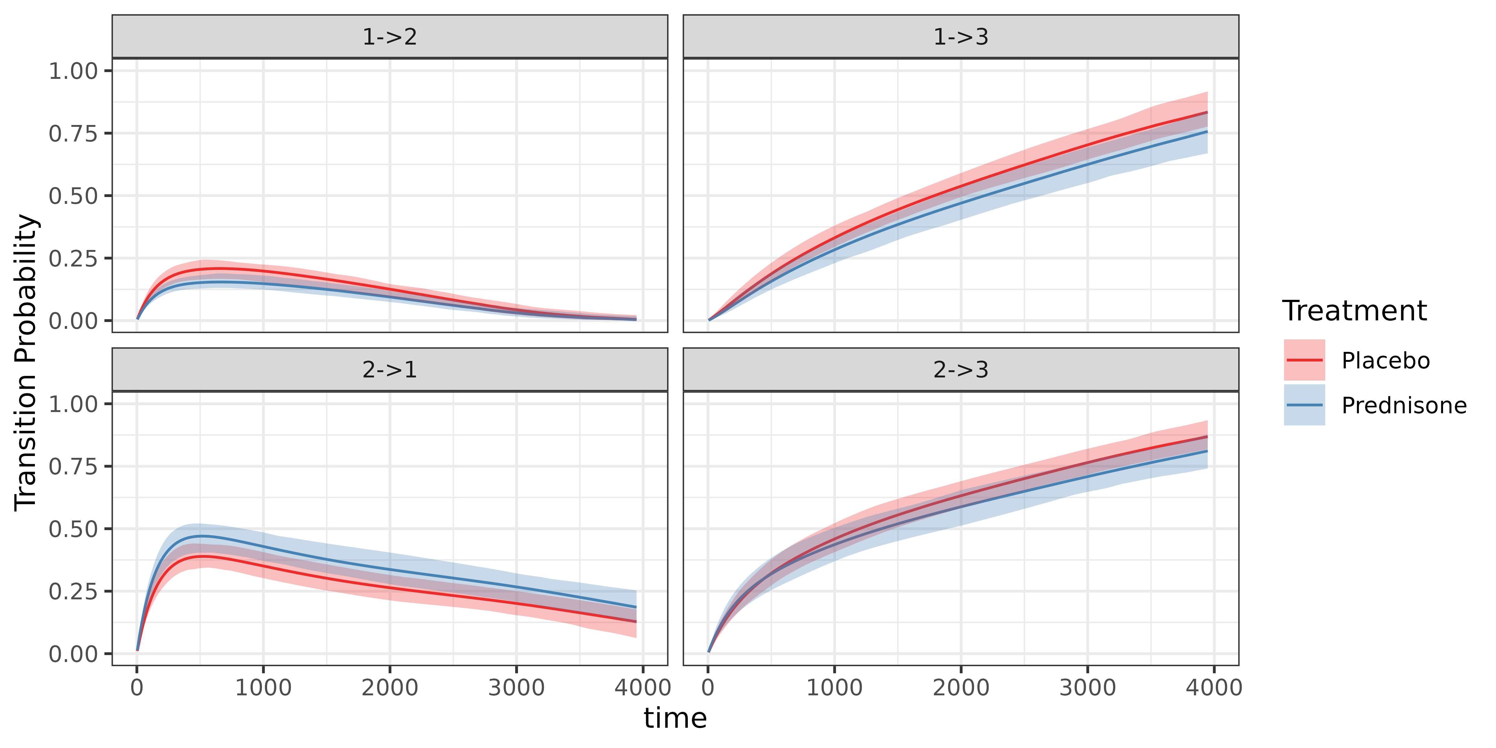

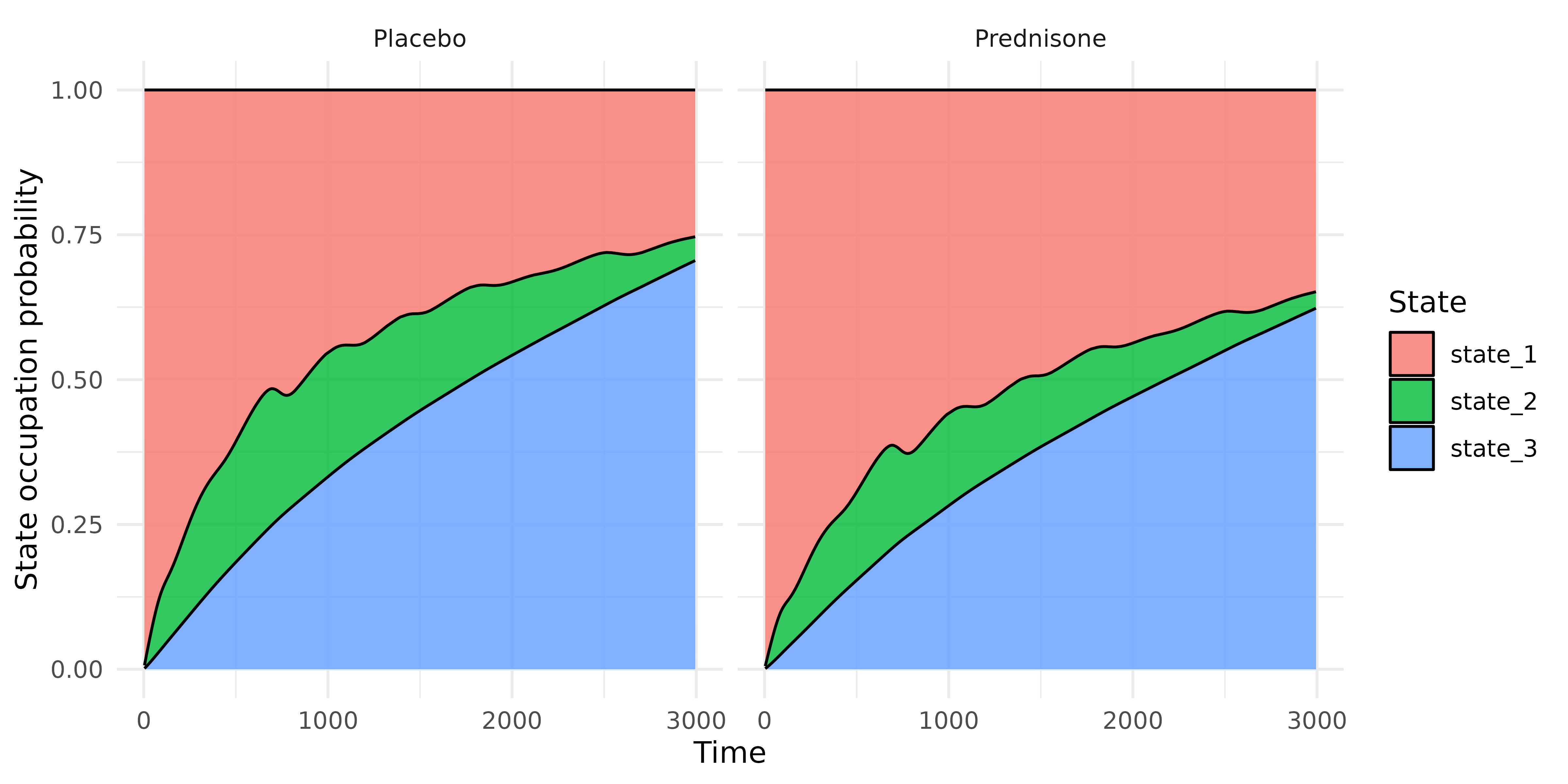
Instead of transition probabilities, one can plot state occupation probabilities using the convenience function gg_state_occupation. State occupation probabilities $\boldsymbol{\pi}(t) = \boldsymbol{\pi}(s) \mathbf{P}(s, t)$ are derived from transition probabilities by assuming an initial state distribution (init_state) $\boldsymbol{\pi}(s)$.

gg_state_occupation(
  ndf, 
  group_var = "treat", 
  init_state = c(1,0,0)
  )

Model Comparisons: Comparison of pammtools results with the mstate Aalen-Johannsen estimator

To validate that the PAMM baseline hazards are correctly specified, we compare cumulative hazards and transition probabilities estimated by pammtools against the non-parametric Aalen-Johannsen estimator from mstate. Since we fit a baseline model without covariates, both approaches should yield identical results up to numerical approximation from the piecewise-constant hazard assumption in PAMMs.

First, we compare the cumulative hazards, which form the basis for all downstream quantities, i.e. here the transition probabilities.

R-Code for comparing mstate models

# --- setup ------------------------------------------------------------------
data(prothr, package = "mstate")
tmat        <- attr(prothr, "trans")
treat_levels <- c("Placebo", "Prednisone")
trans_labels <- c("1->2", "1->3", "2->1", "2->3")
trans_recode <- c("1->2" = "0->1", "1->3" = "0->2", "2->1" = "1->0", "2->3" = "1->2")
alpha        <- 0.05

transitions_to_extract <- list(
  list(from = 1, to = 2, label = "1->2"),
  list(from = 1, to = 3, label = "1->3"),
  list(from = 2, to = 1, label = "2->1"),
  list(from = 2, to = 3, label = "2->3")
)

# --- helpers ----------------------------------------------------------------
fit_msfit <- function(treat_label) {
  pr <- subset(prothr, treat == treat_label)
  attr(pr, "trans") <- tmat
  msfit(coxph(Surv(Tstart, Tstop, status) ~ strata(trans), data = pr), trans = tmat)
}

extract_probtrans <- function(pt, treat_label) {
  z <- qnorm(1 - alpha / 2)
  map_dfr(transitions_to_extract, function(tr) {
    state_col <- paste0("pstate", tr$to)
    se_col    <- paste0("se",     tr$to)
    prob      <- pt[[tr$from]][[state_col]]
    se        <- pt[[tr$from]][[se_col]]
    data.frame(
      tend        = pt[[tr$from]]$time,
      trans_prob  = prob,
      trans_lower = prob - z * se,
      trans_upper = prob + z * se,
      transition  = tr$label
    )
  }) |>
    mutate(treat = treat_label, package = "mstate")
}

# --- fit --------------------------------------------------------------------
msf <- setNames(map(treat_levels, fit_msfit), treat_levels)
pt  <- setNames(map(msf, ~ probtrans(.x, predt = 0)), treat_levels)

# --- cumulative hazards -----------------------------------------------------
long_mstate <- map_dfr(treat_levels, ~ {
  msf[[.x]]$Haz |>
    mutate(transition = trans_labels[trans], treat = .x)
}) |>
  rename(tend = time, cumu_hazard = Haz) |>
  mutate(package = "mstate") |>
  select(tend, treat, transition, cumu_hazard, package)

long_haz_df <- ndf |>
  mutate(package = "pammtools") |>
  select(tend, treat, transition, cumu_hazard, package) |>
  bind_rows(long_mstate) |>
  filter(tend < 3000) |>
  mutate(transition = trans_recode[transition])

# --- transition probabilities -----------------------------------------------
pt_df_mstate <- map_dfr(
  treat_levels,
  ~ extract_probtrans(pt[[.x]], .x)
)

pt_df <- ndf |>
  mutate(package = "pammtools") |>
  select(tend, treat, transition, trans_prob, trans_lower, trans_upper, package) |>
  bind_rows(pt_df_mstate) |>
  filter(tend < 3000)

# --- plotting ---------------------------------------------------------------
p_comparison_cumu_haz <- ggplot(
  long_haz_df, 
  aes(x=tend, y=cumu_hazard, 
      col=treat, 
      linetype = package)
  ) + 
  geom_line() +
  facet_wrap(~transition, ncol = 4, labeller = label_both) +
  scale_color_manual(values = c("firebrick2"
                                , "steelblue")
                     ) +
  ylab("Cumulative Hazards") +
  xlab("time in days") +
  scale_y_continuous(limits = c(0, 6), oob = scales::oob_keep) +
  scale_linetype_manual(values=c("dotted", "solid")) +
  theme_bw()

p_comparison_trans_prob <- ggplot(
  pt_df,
  aes(x = tend, y = trans_prob,
      col      = interaction(package, treat),
      fill     = interaction(package, treat))
) +
  # point estimates
  geom_line(linewidth = 0.7) +
  # pammtools CIs as dotted lines
  geom_line(
    data = subset(pt_df, package == "pammtools"),
    aes(y = trans_lower), linetype = "dotted", linewidth = 0.4
  ) +
  geom_line(
    data = subset(pt_df, package == "pammtools"),
    aes(y = trans_upper), linetype = "dotted", linewidth = 0.4
  ) +
  # mstate CIs as shaded ribbon
  geom_ribbon(
    data = subset(pt_df, package == "mstate"),
    aes(ymin = trans_lower, ymax = trans_upper),
    alpha = 0.2, color = NA
  ) +
  facet_grid(rows = vars(treat), cols = vars(transition), labeller = label_both) +
  scale_color_manual(
    values = c(
      "mstate.Placebo"       = "grey50",
      "mstate.Prednisone"    = "grey50",
      "pammtools.Placebo"    = "firebrick2",
      "pammtools.Prednisone" = "steelblue"
    )
  ) +
  scale_fill_manual(
    values = c(
      "mstate.Placebo"       = "grey70",
      "mstate.Prednisone"    = "grey70",
      "pammtools.Placebo"    = "firebrick2",
      "pammtools.Prednisone" = "steelblue"
    )
  ) +
  scale_y_continuous(limits = c(0, 1), oob = scales::oob_keep) +
  labs(y = "Transition Probability", x = "Time in days") +
  theme_bw() +
  guides(color = "none", fill = "none")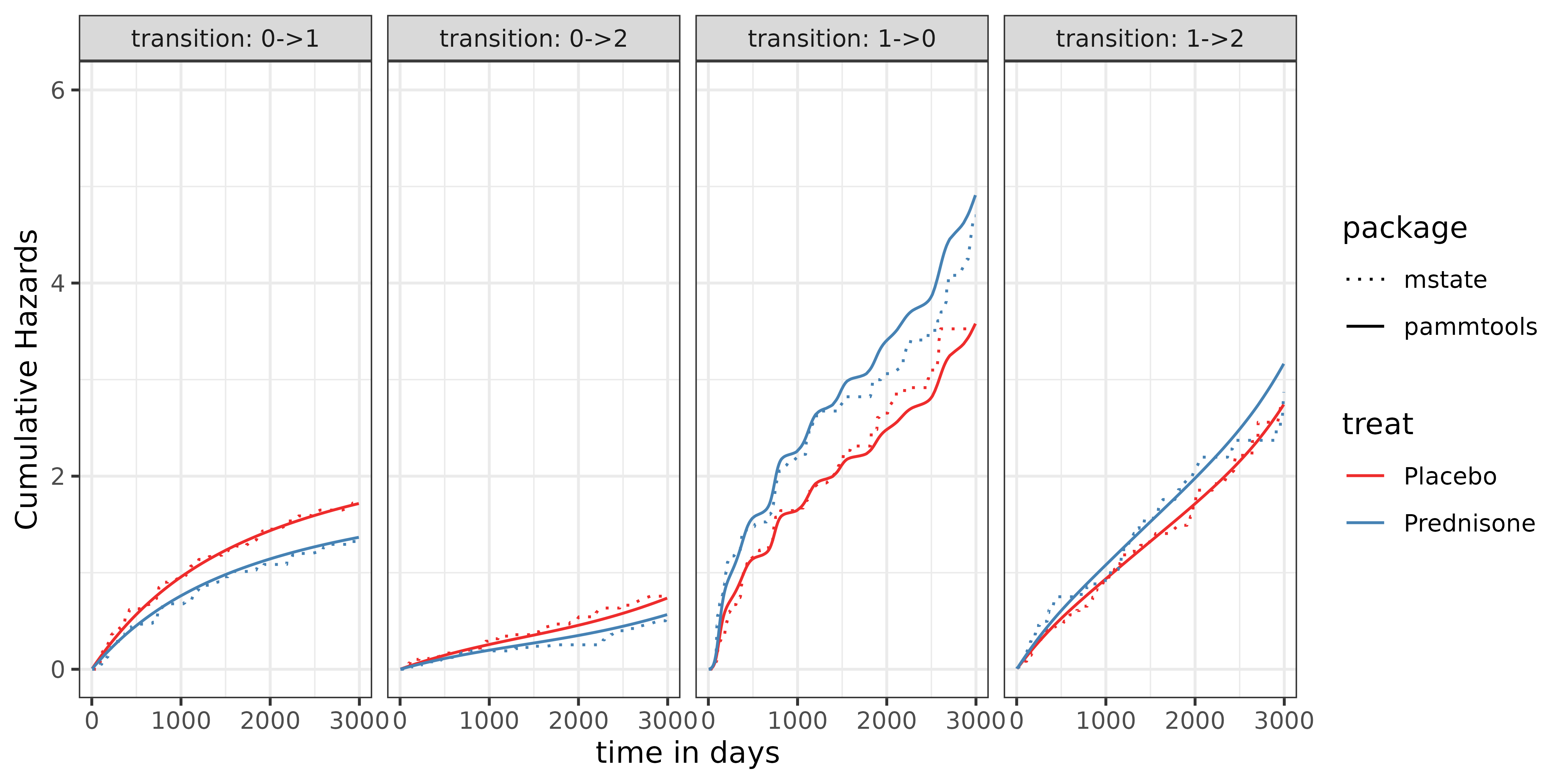

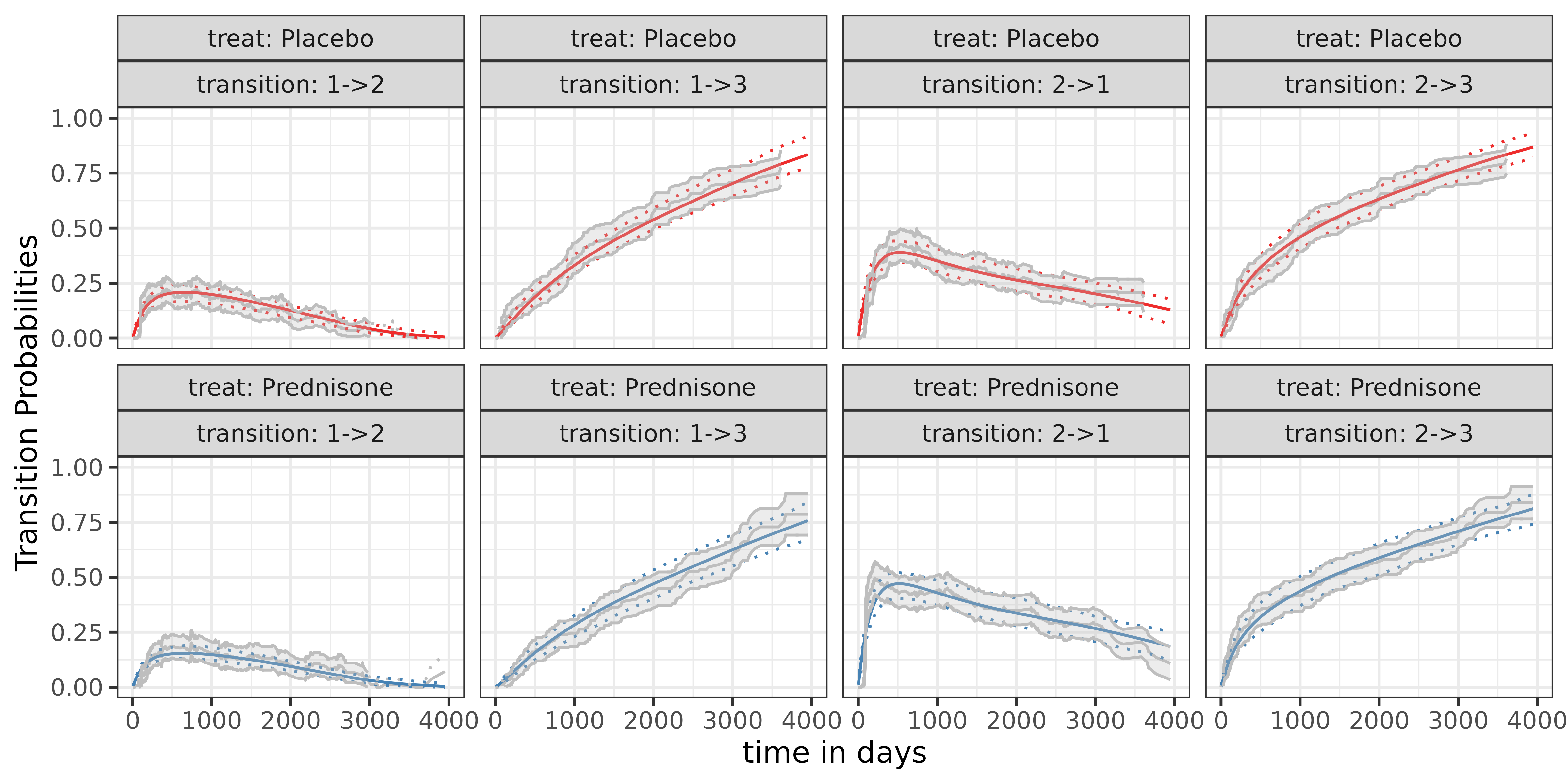
Second, we compare transition probability point estimates and confidence bands. Confidence bands from mstate (shaded ribbon) and pammtools (dotted lines) are overlaid to allow a direct assessment of both location and uncertainty.