Simulating Time-To-Event Data

Andreas Bender, Johannes Piller

2025-08-20

library(tidyr)
library(dplyr)
library(ggplot2)
library(survival)
library(mgcv)
library(pammtools)

theme_set(theme_bw())

For convenience, the pammtools package contains a lightweight, but versatile function for the simulation of time-to-event data, with potentially smooth, smoothly time-varying effects. For the simulation of survival times we use the Piece-wise exponential distribution $t \sim \text{PEXP}(\boldsymbol{\lambda}, \textbf{t})$, which is implemented in the msm package (Jackson 2011). Here $\boldsymbol{\lambda}$ is a vector of hazards at time points $\textbf{t}$ and $\boldsymbol{\lambda}$ can be specified conveniently using a formula notation.

In Section Motivation, we empirically demonstrate that even crude PEXP hazards can be used to simulate survival times from continuous distributions. In Section Flexible, covariate dependent simulation of survival times, we illustrate the simulation of survival times based on hazard rates that flexibly depend on time-constant covariates. Lastly, Section Simulation of survival times with cumulative effects shows how to simulate from hazards with cumulative effects of TDCs.

Motivation

We use a simple Weibull baseline hazard model to illustrate that the function indeed simulates event times from the desired distribution, even though the hazards $\boldsymbol{\lambda}$ are assumed to be piece-wise constant between two time-points in $\textbf{t}$.

# Weibull hazard function
hweibull <- function(t, alpha, lambda) {
  dweibull(t, alpha, lambda)/pweibull(t, alpha, lambda, lower.tail=FALSE)
}

# plot hazard and survival probability:
alpha <- 1.5
lambda <- 10
t <- seq(0, 10, by=.01)
wb_df <- data.frame(t = t) %>%
  mutate(
    hazard   = hweibull(t, alpha, lambda),
    survival = pweibull(t, alpha, lambda, lower.tail = FALSE))

The figure below depicts the hazard rate and survivor function of a Weibull distribution with $T \sim WB(\alpha = 1.5, \lambda = 10)$.

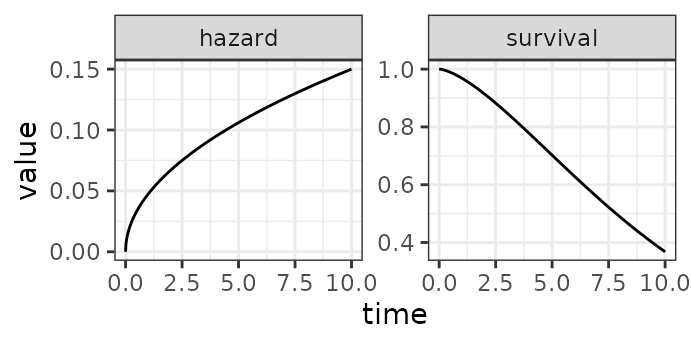
Hazard rate (left) and survivor function (right) of the $WB(1.5, 10)$ distribution.

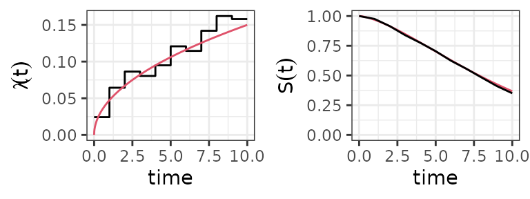
PEM estimates of the baseline hazard $\lambda(t)$ (left panel) and survival probability $S(t)$ (right panel). Red lines indicate the true Weibull hazard and survival probability, respectively.

The figure above (left panel) shows the baseline hazard estimated by a PEM with 10 intervals based on $n=1000$ survival times simulated from $WB(1.5, 10)$. Although the approximation of the underlying smooth hazard is relatively crude, the survival function calculated from this step hazard is very close to the true survivor function (cf. right panel).

Finally, below, we depict the distribution of survival times (Kaplan-Meier estimates) for $n=1000$ survival times simulated directly from the correct Weibull distribution (rweibull(n, 1.5, 10)) on the one hand and from the $PEXP$ distribution (based on the crude hazard) on the other hand.

Comparison of Kaplan-Meier survival probability estimates based on survival times simulated directly from the Weibull distribution $WB(1.5, 10)$ and based on survival times simulated from the $PEXP$ distribution based on the hazards depicted above. The black line indicates the true Weibull survival probability on $t\in [0, 10]$.

Flexible, covariate dependent simulation of survival times

To simulate survival times from the PEXP distribution conveniently, pammtools provides the sim_pexp function. Similar to the as_ped function, it uses a formula interface, which allows to specify complex hazards relatively easily. To start, we simulate data from $$\log(\lambda(t|x_1, x_2)) = -3.5 + f_0(t) -0.5 x_1 + \sqrt{x_2},$$ where $f_0(t)$ is based on the Gamma(8,2) density function. Any existing or previously defined function can be used in the formula argument to sim_pexp. The argument cut defines the time-points at which the piece-wise constant hazard will change its value, for example, the hazard will change its value at $t=1, t=2, \ldots$ with $f_0(t)$ (and other time-varying effects) evaluated at the respective interval end-points. sim_pexp returns the original data augmented by the simulated survival times (time) as well as a status column.

# basic data
set.seed(7042018)
# create data set with covariates
n <-1000
df <- tibble::tibble(x1 = runif(n, -3, 3), x2 = runif(n, 0, 6))
# baseline hazard function
f0 <- function(t) {dgamma(t, 8, 2) * 6}
# simulate data from PEXP
sim_df <- sim_pexp(
  formula = ~ -3.5 + f0(t) -0.5*x1 + sqrt(x2),
  data    = df,
  cut     = 0:10)

We evaluate the simulated data by comparing estimates of the Cox PH model and the PAM estimates.

# for comparison, estimate with Cox PH
mod_cph <- coxph(Surv(time, status) ~ x1 + pspline(x2), data=sim_df)
# and using PAMs
ped <- split_data(Surv(time, status)~., data = sim_df, cut = seq(0, 10))
 
mod_pam <- gam(
  formula = ped_status ~ s(tend) + x1 + s(x2),
  data    = ped,
  family  = poisson,
  offset  = offset)
cbind(PAM = coef(mod_pam)[2] , COX = coef(mod_cph)[1])

##           PAM        COX
## x1 -0.5573143 -0.5578749

Note that the simulation could be easily extended to contain time-varying effects, e.g. by defining a function

f_tx <- function(t, x) sqrt(x)*log(t)

and calling

sim_pexp(~ -3.5 + f0(t) -0.5*x1 + f_tx(t, x2), data = df, cut = 0:10)

Simulation of survival times with cumulative effects

Weighted cumulative exposure

In this section we demonstrate how to simulate data with hazard rates

$$\log(\lambda(t|x_1, x_2, \textbf{z})) = -3.5 + f_0(t) -0.5 x_1 + \sqrt{x_2} + \int_{\mathcal{T}(t)} h(t-t_z)z(t_z) \text{d}t_z.$$

which constitutes a so-called weighted cumulative exposure model (Sylvestre and Abrahamowicz 2009). The static part of the data set as well as the baseline hazard and TCC effects are identical to the previous section. For the cumulative effect, we define the exposure time grid (i.e., the time points $t_z$ at which the TDC was observed) and use the function add_tdc (mnemonic: add time-dependent covariate) to add the information on the exposure times and the $z(t_z)$ to the data.

## [[1]]
##  [1] -5.00 -4.75 -4.50 -4.25 -4.00 -3.75 -3.50 -3.25 -3.00 -2.75 -2.50 -2.25
## [13] -2.00 -1.75 -1.50 -1.25 -1.00 -0.75 -0.50 -0.25  0.00  0.25  0.50  0.75
## [25]  1.00  1.25  1.50  1.75  2.00  2.25  2.50  2.75  3.00  3.25  3.50  3.75
## [37]  4.00  4.25  4.50  4.75  5.00

The partial effect $h(t-t_z)z(t_z)$ (see function f_wce) and the lag-lead window $\mathcal{T}(t)$ (see function ll_fun) are defined and depicted below.

The left panel of the figure shows the latency-dependent weight function $h(t-t_z)$ for the exposures $z(t_z)$. The middle panel shows the lag-lead window with partial effects. Note that $h(t-t_z)$ only depends on the latency, not the specific combination of $t$ and $t_z$. The right panel shows that the cumulative effect $g(\textbf{z}, t)$ varies over $t$ even for constant exposure $z(t_z) = z$ since it is integrated over different windows of effectiveness $\mathcal{T}(t)$.

# define lag-lead function: integrate over the preceding 12 time units
ll_fun <- function(t, tz) ((t - tz) >= 0) & ((t - tz) <=  12)
# gg_laglead(0:10, -5:5, ll_fun)

# partial effect h(t - tz) * z
f_wce <- function(t, tz, z) {
  0.5 * (dnorm(t - tz, 6, 2.5)) * z
}

Expand here to see R-Code

LL_df  <- get_laglead(0:10, -5:5, ll_fun)
LL_df <- LL_df %>%
  mutate(latency = t - tz,
         partial = f_wce(t, tz, z = 1)) %>%
  filter(t != 0)

gg_partial <- LL_df %>% filter(LL!=0) %>%
  ggplot(aes(x = t - tz, y = partial)) +
  geom_line() +
  ylab(expression(h(t - t[z]))) + xlab(expression(t - t[z]))

LL_df$partial[LL_df$LL == 0] <- NA
gg_partial_LL <- ggplot(LL_df,
                        aes(x = t, y = tz, fill = partial * LL, z = partial * LL)) +
  scale_x_continuous(expand = c(0, 0)) +
  scale_y_continuous(name = expression(t[z]), expand = c(0, 0)) +
  geom_tile(colour = NA) +
  scale_fill_gradient2(name = expression(h(t - t[z])),
                       na.value = "grey30", low = "steelblue", high = "firebrick2")

gg_cumeff <- LL_df %>%  group_by(t) %>%
  summarize(g_z = sum(partial*LL, na.rm=T)) %>%
  ggplot(aes(x = t, y = g_z)) +
  geom_line() +
  ylab(expression(g(bold(z) == 1, t))) +
  ylim(c(.2, .6))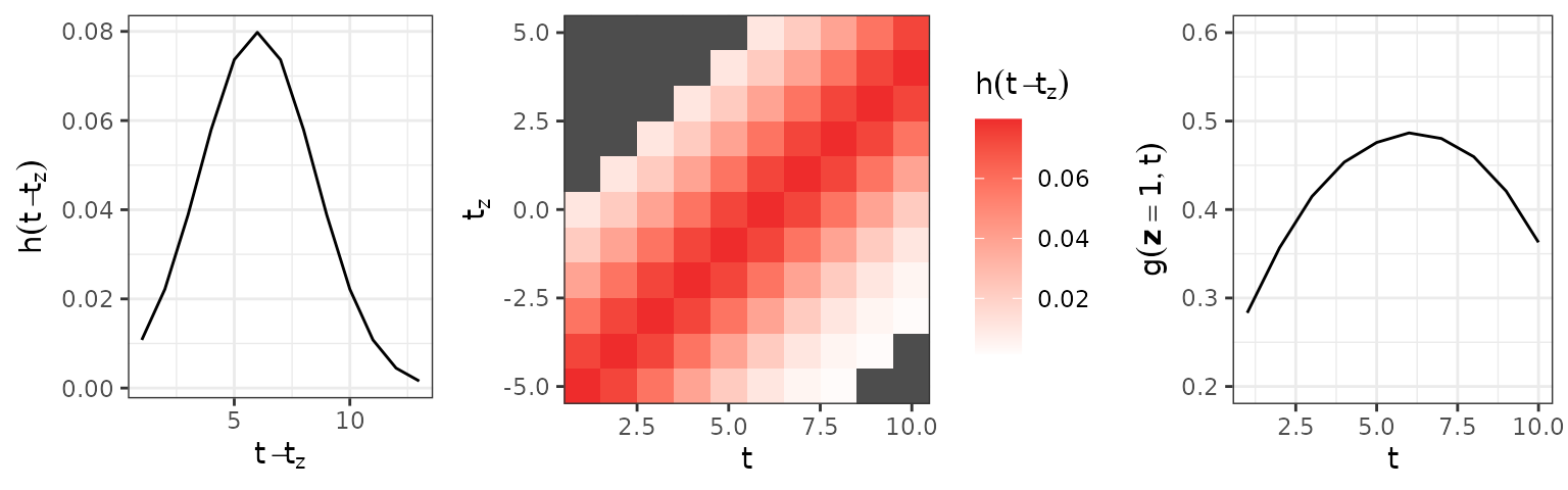

Left: Partial effect $h(t-t_z)$ for different latencies $t-t_z$. Middle: The lag-lead window $\mathcal{T}(t)$ and respective partial effects for each combination of $t$ and $t_z$. Combinations of $t$ and $t_z$ outside the specified lag-lead window in dark gray. Partial effects of exposures at different time-points $t$, $t_z$ are the same if the latency $t-t_z$ is the same, i.e. $h(5-1) = h(6-2) = h(4)$. Right: Cumulative effect $g( extbf{z},t)$ for constant $z(t_z)=1, orall t_z$.

Given the above setup with cumulative effects $g(\textbf{z},t)=\int_{\mathcal{T}(t)}h(t-t_z)z(t_z) \text{d}t_z$, we can now simulate the data using the sim_pexp function.

simdf_wce <- sim_pexp(
  formula = ~ -3.5 + f0(t) -0.5*x1 + sqrt(x2)|
  fcumu(t, tz, z.tz, f_xyz=f_wce, ll_fun=ll_fun),
  data = df, cut = time_grid
  )

Bivariate, smooth partial effects

In this section, we illustrate an extension of the previous simulation, where the exposure $z(t_z)$ affects the hazard non-linearly $$\log(\lambda(t|x_1, x_2, \textbf{z})) = -3.5 + f_0(t) -0.5 x_1 + \sqrt{x2} + \int_{\mathcal{T}(t)} h(t-t_z,z(t_z)) \text{d}t_z$$

Using the sim_pexp function, we can extend the previous simulation by changing the partial effect function (function f_dlnm). The figure below depicts the bivariate, smooth partial effect $h(t-t_z, z(t_z))$ and the resulting cumulative effects $g(\textbf{z},t)$ for a simplified exposure history with constant $z(t_z)=1$ for all $t_z$.

# partial effect h(t - tz) * z
f_dlnm <- function(t, tz, z) {
   20 * ((dnorm(t - tz, 6, 2.5)) * (dnorm(z, 1.25, 2.5) - dnorm(-1, 1.25, 2.5)))
}

simdf_dlnm <- sim_pexp(
  formula = ~ -4.5 + f0(t) -0.5*x1 + sqrt(x2)|
     fcumu(t, tz, z.tz, f_xyz=f_dlnm, ll_fun=ll_fun),
  data = df, cut = time_grid)

Expand here to see R-Code

viz_df <- get_laglead(time_grid, tz, ll_fun = ll_fun) %>%
combine_df(data.frame(z = seq(-3, 3, by = 0.25))) %>%
mutate(
  latency = t - tz,
  partial = f_dlnm(t, tz, z))

gg_partial_dlnm <- viz_df %>% filter(t == 6) %>% filter(LL == 1) %>%
  ggplot(aes(x = z, y = latency, z = partial)) +
  geom_tile(aes(fill=partial)) +
  scale_y_reverse() +
  scale_fill_gradient2(name = expression(h(t-t[z])),
                       low = "steelblue", high="firebrick2")+
  geom_contour(col = "grey30") +
  ylab(expression(t-t[z])) + xlab(expression(z))
gg_z_dlnm <- viz_df %>% filter(z %in% c(1)) %>%
  group_by(t, z) %>%
  summarize(g_z = sum(0.25*partial)) %>%
  ungroup() %>%
  ggplot(aes(x=t, y = g_z)) +
  geom_line()

## `summarise()` has grouped output by 't'. You can override using the `.groups`
## argument.

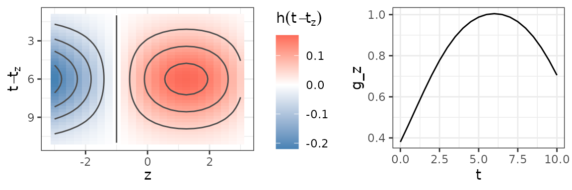
Left: Partial effect $h(t-t_z, z(t_z))$ used for the simulation of survival times. Right: The cumulative effects $g( extbf{z},t)$ resulting from constant exposure histories $z(t_z)=1, \forall t_z$.

Bivariate smooth of time and exposure time

In this subsection, we simulate the data with hazard $$\log(\lambda(t|x_1, x_2, \textbf{z})) = -3.5 + f_0(t) -0.5 x_1 + \sqrt{x_2} + \int_{\mathcal{T}(t)} h(t,t_z)z(t_z)\text{d} t_z.$$ Using the sim_pexp function, we can again extend the previous simulation with the updated partial effect function f_elra.

# partial effect h(t,tz) * z
f_elra <- function(t, tz, z) {
   5*(-(dnorm(tz, -1, 2.5)) * (dnorm(t, 5, 1.5) - dnorm(5, 5, 1.5)))*z
}

simdf_tv_wce <- sim_pexp(formula = ~ -4.5 + f0(t) -0.5*x1 + sqrt(x2)|
     fcumu(t, tz, z.tz, f_xyz = f_elra, ll_fun = ll_fun),
  data = df, cut = time_grid)

Expand here to see R-Code

LL_df_elra <- get_laglead(seq(0,10, by=0.25), seq(-5, 5, by=0.25), ll_fun) %>%
  mutate(partial = f_elra(t, tz, z = 1)) %>%
   filter(LL == 1)
cumu_df_elra <- LL_df_elra %>%
  group_by(t) %>%
  summarize(cumu_eff = sum(0.25*partial))

p_partial_elra_truth <- ggplot(LL_df_elra, aes(x = t, y = tz, z = partial)) +
    geom_tile(aes(fill = partial)) +
    scale_x_continuous(expand=c(0,0)) +
    scale_y_continuous(expand = c(0,0)) +
    scale_fill_gradient2(name = expression(h(t,t[z])),
      low = "steelblue", high = "firebrick2") +
    geom_contour(col = "grey30") +
    ylab(expression(t[z]))

p_cumu_elra_truth <- ggplot(cumu_df_elra, aes(x=t, y = cumu_eff)) +
  geom_line() +
  ylab(expression(g(bold(z), t)))

The figure below depicts the bivariate, smooth partial effect $h(t, t_z)$ (left panel) and the resulting cumulative effect $g(\textbf{z},t)$ for a simplified exposure history with $z(t_z)=1 \forall t_z$ (right panel).

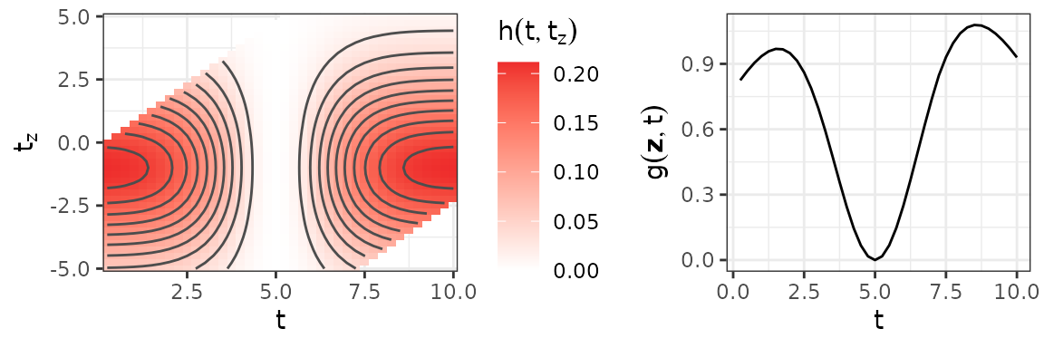
Left: Bivariate partial effect surface $h(t, t_z)$, combinations of $t$ and $t_z$ that lie outside the lag-lead window $\mathcal{T}(t)$ are omitted. Right: The cumulative effect resulting from the partial effect depicted in the left panel for a simplified exposure profile with $z(t_z)=1, \forall t_z$.

References

Jackson, Christopher. 2011. “Multi-State Models for Panel Data: The Msm Package for r.” Journal of Statistical Software 38 (8): 1–28. https://doi.org/10.18637/jss.v038.i08.

Sylvestre, Marie-Pierre, and Michal Abrahamowicz. 2009. “Flexible Modeling of the Cumulative Effects of Time-Dependent Exposures on the Hazard.” Statistics in Medicine 28 (27): 3437–53. https://doi.org/10.1002/sim.3701.