Bayesian Baseline PAMMs: mgcv, jagam, and brms

Show package setup

library(dplyr)
library(ggplot2)
library(mgcv)
library(pammtools)
library(survival)
library(tidyr)
library(tibble)

theme_set(theme_bw())

This vignette compares baseline cumulative hazard estimates from:

a default frequentist PAMM fit with mgcv,
a Bayesian PAMM fit via mgcv::jagam (Wood 2016), which generates JAGS (Plummer 2003) code from the GAM specification and samples it with rjags,
a Bayesian PAMM fit via brms (Bürkner 2017) (which compiles the model to Stan).

All models use the same spline basis for the baseline hazard, and we compare them against the Nelson-Aalen estimate and against each other on a common time grid.

Build note. The JAGS and Stan fits run on an ~11,600-row piece-wise exponential data set and take 15–20 minutes combined – too slow to evaluate on every build. The model-fitting and prediction code below is therefore shown but not executed (eval = FALSE); it is run once by vignettes/precompute_bayesian.R, which saves the resulting pred_df to bayesian_results.rds. The plots and tables below are rendered live from that saved data frame. Running rjags additionally needs a JAGS installation, and brms needs a working Stan toolchain.

Data preparation

data("tumor")
tumor <- tumor %>%
  slice(1:200) %>%
  mutate(id = row_number())

base_df <- basehaz(coxph(Surv(days, status) ~ 1, data = tumor), centered = FALSE) %>%
  rename(nelson_aalen = hazard)

ped <- as_ped(tumor, Surv(days, status) ~ 1, id = "id")

Model fits

1) Default PAMM (`mgcv`)

pam_mgcv <- mgcv::gam(
  formula = ped_status ~ s(tend, k = 20),
  data = ped,
  family = poisson(),
  offset = offset,
  method = "REML"
)

2) Bayesian PAMM via `jagam` + `rjags`

set.seed(101)

jagam_file <- tempfile(fileext = ".jags")
pam_jagam_prep <- mgcv::jagam(
  formula = ped_status ~ s(tend, k = 20),
  data = ped,
  family = poisson(),
  offset = offset,
  file = jagam_file,
  sp.prior = "gamma",
  diagonalize = TRUE
)

library(rjags)
rjags::load.module("glm")
jagam_sampler <- rjags::jags.model(
  file = jagam_file,
  data = pam_jagam_prep$jags.data,
  inits = pam_jagam_prep$jags.ini, # data-driven starts from the penalised GAM
  n.chains = 2,
  quiet = FALSE
)

jagam_post <- rjags::jags.samples(
  model = jagam_sampler,
  variable.names = c("b", "lambda"),
  n.iter = 4000,
  thin = 10
)

pam_jagam <- mgcv::sim2jam(jagam_post, pam_jagam_prep$pregam)

3) Bayesian PAMM via `brms`

library(brms)
set.seed(101)

# The PED has many rows, so each Stan iteration is comparatively expensive;
# running the two chains on separate cores and starting from `init = 0`
# (a hazard of ~1 before the offset) gives a stable, reasonably quick fit.
pam_brms <- brms::brm(
  formula = ped_status ~ s(tend, k = 20) + offset(offset),
  data = ped,
  family = poisson(),
  chains = 2,
  cores = 2,
  iter = 3000,
  warmup = 750,
  init = 0,
  seed = 101,
  refresh = 0,
  silent = 1
)
summary(pam_brms)
brms::pp_check(pam_brms) +
  labs(title = "Posterior predictive check")

Common prediction pipeline

All three models are now driven through the same add_cumu_hazard() call. For mgcv and jagam this uses the analytic (coefficient-based) confidence intervals as before. For brms we make the fit a first-class pammtools backend by defining the two primitives of the unified inference interface – get_hazard() (point hazard) and sim_hazard() (matrix of posterior hazard draws). Once those exist, add_cumu_hazard(ci_type = "sim") builds the cumulative hazard and its posterior credible interval from them, so no manual cumsum/quantile bookkeeping is needed. This is exactly the mechanism the xgboost backend vignette uses for a tree ensemble.

conf_level <- 0.95

newdata_base <- make_newdata(ped, tend = sort(unique(ped$tend))) %>%
  arrange(tend)

method_labels <- c(
  mgcv = "PAMM (mgcv)",
  jagam = "Bayesian PAMM (jagam)",
  brms = "Bayesian PAMM (brms)"
)

# brms as a pammtools backend: the two primitives the unified inference
# interface needs. `sim_hazard()` returns one column per posterior draw; setting
# the offset to 0 yields the bare hazard rate (exp(eta) without the
# log-interval-length term), which `add_cumu_hazard()` then multiplies by the
# interval length itself.
sim_hazard.brmsfit <- function(object, newdata, nsim = NULL, ...) {
  newdata$offset <- 0
  ep <- brms::posterior_epred(
    object,
    newdata = newdata,
    summary = FALSE,
    re_formula = NA
  )
  t(as.matrix(ep)) # rows = time points, cols = posterior draws
}
get_hazard.brmsfit <- function(object, newdata, ...) {
  rowMeans(sim_hazard.brmsfit(object, newdata, ...))
}

get_cumu <- function(model, method_id, newdata, conf_level = 0.95) {
  # jam (jagam posterior) objects need to advertise the gam/glm/lm classes so
  # that the analytic CI machinery and design-matrix extraction dispatch.
  if (inherits(model, "jam")) {
    class(model) <- unique(c(class(model), "gam", "glm", "lm"))
  }
  # brms has no coefficient covariance -> simulation CIs from posterior draws;
  # mgcv/jagam keep their analytic (coefficient-based) CIs.
  ci_type <- if (inherits(model, "brmsfit")) "sim" else "default"
  pred <- add_cumu_hazard(
    newdata,
    model,
    ci = TRUE,
    ci_type = ci_type,
    se_mult = stats::qnorm((1 + conf_level) / 2),
    alpha = 1 - conf_level,
    # boundary = FALSE keeps all methods on the identical `tend` grid: the
    # default would prepend a t = 0 row for gam/jagam but not for brms, which
    # would misalign the curves and the downstream comparison join.
    boundary = FALSE
  )

  tibble::tibble(
    tend = pred$tend,
    method_id = method_id,
    method = unname(method_labels[method_id]),
    cumu_hazard = pred$cumu_hazard,
    cumu_lower = pred$cumu_lower,
    cumu_upper = pred$cumu_upper
  )
}

pred_df <- bind_rows(
  get_cumu(pam_mgcv, "mgcv", newdata_base, conf_level = conf_level),
  get_cumu(pam_jagam, "jagam", newdata_base, conf_level = conf_level),
  get_cumu(pam_brms, "brms", newdata_base, conf_level = conf_level)
)

Reshape for comparison

# Guard against a stale `bayesian_results.rds`: the comparison below joins the
# precomputed `pred_df` to the live `newdata_base` grid by position, so the two
# grids must match. Fail loudly if the precompute is out of sync with the Rmd.
stopifnot(identical(
  sort(unique(pred_df$tend)),
  sort(unique(newdata_base$tend))
))

na_on_grid <- stats::approx(
  x = base_df$time,
  y = base_df$nelson_aalen,
  xout = newdata_base$tend,
  method = "constant",
  f = 0,
  rule = 2
)$y

pred_wide <- pred_df %>%
  select(tend, method_id, cumu_hazard) %>%
  pivot_wider(names_from = method_id, values_from = cumu_hazard) %>%
  mutate(nelson_aalen = na_on_grid)

method_ids <- c("mgcv", "jagam", "brms")
pairwise_combos <- utils::combn(method_ids, 2, simplify = FALSE)

Visual comparison to Nelson-Aalen

Plotting code

ggplot(pred_df, aes(x = tend, y = cumu_hazard, color = method, fill = method, linetype = method)) +
  geom_ribbon(aes(ymin = cumu_lower, ymax = cumu_upper), alpha = 0.18, color = NA) +
  geom_line(linewidth = 0.75) +
  geom_stephazard(
    data = base_df,
    aes(x = time, y = nelson_aalen),
    inherit.aes = FALSE,
    color = "black",
    linetype = 2
  ) +
  labs(
    x = "time",
    y = expression(hat(Lambda)(t)),
    title = "Baseline cumulative hazard comparison",
    subtitle = "Dashed black curve: Nelson-Aalen reference"
  ) +
  theme(legend.position = "bottom")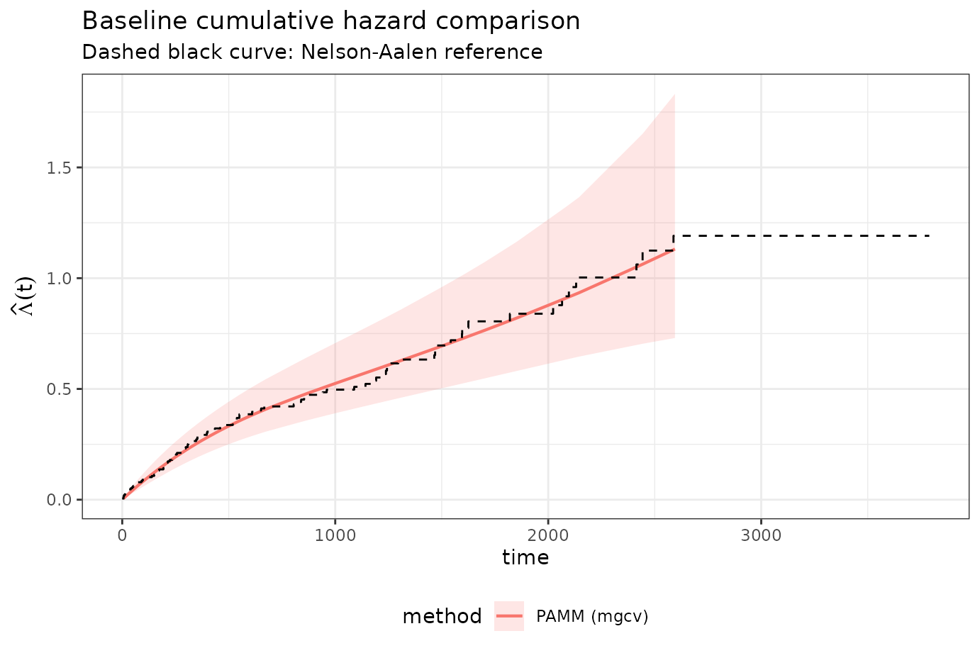

Numeric comparisons

Table code

cmp_na_tbl <- bind_rows(lapply(method_ids, function(method_id) {
  diff <- pred_wide[[method_id]] - pred_wide$nelson_aalen
  tibble(
    method = method_labels[[method_id]],
    rmse_vs_nelson_aalen = sqrt(mean(diff^2)),
    max_abs_diff_vs_nelson_aalen = max(abs(diff))
  )
}))

knitr::kable(cmp_na_tbl, digits = 4)

method	rmse_vs_nelson_aalen	max_abs_diff_vs_nelson_aalen
PAMM (mgcv)	0.0209	0.0684
Bayesian PAMM (jagam)	0.0765	0.1572
Bayesian PAMM (brms)	0.0190	0.0637

Table code

cmp_pairwise_tbl <- bind_rows(lapply(pairwise_combos, function(ids) {
  lhs <- ids[[1]]
  rhs <- ids[[2]]
  diff <- pred_wide[[lhs]] - pred_wide[[rhs]]
  tibble(
    contrast = paste0(method_labels[[lhs]], " - ", method_labels[[rhs]]),
    rmse = sqrt(mean(diff^2)),
    max_abs_diff = max(abs(diff))
  )
}))
knitr::kable(cmp_pairwise_tbl, digits = 4)

contrast	rmse	max_abs_diff
PAMM (mgcv) - Bayesian PAMM (jagam)	0.0738	0.1090
PAMM (mgcv) - Bayesian PAMM (brms)	0.0029	0.0062
Bayesian PAMM (jagam) - Bayesian PAMM (brms)	0.0737	0.1128

References

Bürkner, Paul-Christian. 2017. “brms: An R Package for Bayesian Multilevel Models Using Stan.” Journal of Statistical Software 80 (1): 1–28. https://doi.org/10.18637/jss.v080.i01.

Plummer, Martyn. 2003. “JAGS: A Program for Analysis of Bayesian Graphical Models Using Gibbs Sampling.” In Proceedings of the 3rd International Workshop on Distributed Statistical Computing (DSC 2003), edited by Kurt Hornik, Friedrich Leisch, and Achim Zeileis. Vienna, Austria. https://www.r-project.org/conferences/DSC-2003/Proceedings/Plummer.pdf.

Wood, Simon N. 2016. “Just Another Gibbs Additive Modeler: Interfacing JAGS and mgcv.” Journal of Statistical Software 75 (7): 1–15. https://doi.org/10.18637/jss.v075.i07.

2026-06-17