Interval-Censored Data

library(pammtools)
library(survival)
library(dplyr)
library(ggplot2)

Background

In many studies the event time is not observed exactly but only known to lie in an interval $(L_i, R_i]$ – for example because subjects are examined at a sequence of inspection times and we only learn that the event happened between the last clean and the first positive visit. This is interval censoring.

A piecewise-exponential additive model (PAMM) assumes a piecewise-constant hazard, so the conditional distribution of the event time within $(L_i, R_i]$ is known in closed form. pammtools exploits this with a multiple imputation (MI) strategy (Pan 2000): exact event times are repeatedly drawn from $p(T \mid L_i < T \le R_i, x_i, \theta)$ , each completed data set is transformed and re-fit with the standard right-censored pipeline, and the fits are pooled for inference following Rubin’s rules (Rubin 1987). Naive midpoint imputation, by contrast, typically yields reasonable point estimates but invalid (too narrow) confidence intervals. Related model-based imputation schemes for the interval-censored hazard are discussed by Bebchuk and Betensky (2000); the icenReg package (Anderson-Bergman 2017) provides non-parametric and parametric alternatives that are useful as a cross-check.

Interval-censored data are specified through the usual survival interface, Surv(L, R, type = "interval2"), where L == R denotes an exact time, R == Inf a right-censored observation, L == 0 a left-censored one, and 0 < L < R < Inf a genuine interval.

Simulating interval-censored data

add_inspections() turns exact simulated times (here from sim_pexp()) into interval-censored panel data by drawing (per-subject, by default) inspection times. The true event time is retained in true_time so we can check our work.

Here a binary covariate trt acts through a time-varying effect that is absent at baseline and grows over follow-up. The control group (trt == 0) has a constant hazard; the other group starts at the same hazard but its log-hazard then rises linearly in time – the log-hazard ratio is 0.15 * t, zero at t = 0 – so the two hazards start together and fan apart, an increasingly harmful effect and a clear departure from proportional hazards. Because factors enter the (numeric) linear predictor directly, the effect is written with an explicit indicator (trt == 1).

The inspection rate controls how much information the interval censoring destroys: a dense grid pins each event down tightly and leaves little to impute, a sparse one brackets events only loosely. We use a moderate schedule (rate = 1.5, mean inter-inspection gap $2/3$ ) – dense enough that these simple hazards are recovered well, yet still leaving each event bracketed in an interval that straddles several analysis cut-points, so the gap between proper MI and naive midpoint intervals stays appreciable.

set.seed(3)
df  <- data.frame(trt = rbinom(1000, 1, 0.5) |> as.factor())
sdf <- sim_pexp(~ -2.2 + 0.15 * t * (trt == "1"), df,
                cut = seq(0, 10, by = 0.1))
icd <- add_inspections(sdf, rate = 1.5, max_time = 10)
icd %>% select(id, trt, true_time, L, R) %>% head()

## # A tibble: 6 × 5
##      id trt   true_time     L      R
##   <int> <fct>     <dbl> <dbl>  <dbl>
## 1     1 0         10    10    Inf   
## 2     2 1          6.89  6.87   7.33
## 3     3 0         10    10    Inf   
## 4     4 0         10    10    Inf   
## 5     5 1          3.98  3.96   4.31
## 6     6 1          3.78  3.21   3.78

Fitting a PAMM by multiple imputation

pamm_ic() runs the whole MI workflow: an initial midpoint fit, then m rounds of (proper) imputation and re-fitting on a fixed interval grid.

We give each group its own smooth log-baseline-hazard via s(tend, by = trt) (a factor by-variable yields one centred smooth per level) plus the parametric trt main effect for the overall level difference between groups.

fit <- pamm_ic(
  Surv(L, R, type = "interval2") ~ trt,
  data          = icd,
  model_formula = ped_status ~ trt + s(tend, by = trt),
  cut           = seq(0, 10, by = 0.5),
  m             = 20
)
fit

## Piecewise exponential additive model for interval-censored data
##   via multiple imputation (20 proper imputations)
##   task        : single event
##   model       : ped_status ~ trt + s(tend, by = trt)
##   subjects    : 1000 (809 interval/left-censored)
##   cut-points  : 21 breaks in [0, 10]
## 
## Use summary() for pooled inference and add_*() for pooled quantities of interest.

print() gives a compact overview; summary() reports the pooled inference: parametric coefficients and covariances are combined with Rubin’s rules (so the reported standard errors include the between-imputation variability), term p-values use the median-p rule (Bolt et al. 2022), and the fraction of missing information induced by the interval censoring is reported as well.

summary(fit)

## Pooled PAMM summary (multiple imputation for interval-censored data)
## 
## Task           : single event 
## Family         : poisson 
## Model          : ped_status ~ trt + s(tend, by = trt) 
## Imputations    : 20 (proper) 
## Subjects       : 1000 ( 809 interval/left-censored ); PED rows per fit: 11042 
## 
## Parametric coefficients (Rubin-pooled estimates & SEs, median-p):
##             Estimate Std. Error z value Pr(>|z|)    
## (Intercept)  -2.1743     0.0559  -38.91  < 2e-16 ***
## trt1          0.5358     0.0730    7.34  1.4e-13 ***
## ---
## Signif. codes:  0 '***' 0.001 '**' 0.01 '*' 0.05 '.' 0.1 ' ' 1
## 
## Approximate significance of smooth terms (mean edf, median-p over imputations):
##               edf Ref.df statistic p-value    
## s(tend):trt0 1.72   1.98      0.96    0.79    
## s(tend):trt1 1.00   1.00     82.19  <2e-16 ***
## ---
## Signif. codes:  0 '***' 0.001 '**' 0.01 '*' 0.05 '.' 0.1 ' ' 1
## 
## Fraction of missing information (FMI):
## Parametric coefficients:
##               FMI
## (Intercept) 0.003
## trt1        0.008
## 
## Smooth terms (five-number summaries over training PED rows):
##                Min    Q1 Median    Q3   Max
## s(tend):trt0 0.013 0.013  0.029 0.171 0.591
## s(tend):trt1 0.024 0.024  0.039 0.039 0.039
## 
## Standard errors include within- + between-imputation variance (Rubin's rules);
## p-values are medians over imputations.

The m imputation fits are stored in fit$fits in a slimmed form (the per-observation slots are dropped, so memory does not grow with the data set size), and pooled summary diagnostics live in fit$pooled. Because smooth bases can differ across imputed data sets, fit$pooled is not a single gam object for direct predict() or plot() calls. The pooled add_*() methods below operate on the imputation fits directly: they combine the per-imputation posterior draws so the intervals reflect both within- and between-imputation uncertainty.

The fraction of missing information (FMI) is a Rubin-style diagnostic for how much of an estimate’s uncertainty is due to the unobserved exact event times. For a scalar quantity $Q$ , write $W$ for the average within-imputation variance and $B$ for the between-imputation variance of the point estimates. The relative increase in variance is $(1 + 1/m)B/W$ , and the FMI is the corresponding fraction of the total uncertainty attributable to the missing information (with the usual small-sample correction for finite m). Values near zero mean that interval censoring adds little uncertainty for that quantity; values near one mean the imputed event times dominate the uncertainty. summary() reports this for the parametric coefficients, and for smooth terms it reports five-number summaries over the training PED grid. Below we compute the same diagnostic directly for the hazard rate, point-by-point on the plotting grid.

FMI is also useful for choosing the number of imputations. Small values of m such as 5 or 10 are fine while developing the model, but reported analyses should usually start around m = 20. If the reported FMI values are mostly below 0.10, that is often enough; if they are around 0.10–0.30, use roughly 30–50 imputations; if they are around 0.30–0.50, use roughly 50–100; and if they are larger than 0.50, use at least 100 and check sensitivity to a larger m or a different random seed. The classical relative-efficiency approximation, $(1 + \lambda/m)^{-1}$ for FMI $\lambda$ , explains why moderate m can already be efficient on average, but plotted smooths and interval endpoints can still show Monte Carlo noise. Keep this separate from nsim: m controls imputation uncertainty, whereas nsim controls the simulation noise in posterior-draw intervals for plotted quantities of interest.

We compare two PAMM estimates per group. The MI estimate pools the imputation fits, so its intervals carry both the within-fit and the between-imputation uncertainty. The midpoint estimate is the initialiser fit (fit$init_fit): a single PAMM fit to the interval midpoints, which treats those imputed times as if observed. We request simulation-based intervals (ci_type = "sim") for the midpoint fit so that both estimates use the same (proper) interval machinery as the pooled pamm_ic methods – the pooled methods always simulate from each fit’s posterior, so this is a like-for-like comparison that differs only by the between-imputation variance. (The default ci_type = "default" instead cumulates the pointwise hazard limits, which yields a noticeably more conservative band.)

ped <- as_ped(icd, Surv(L, R, type = "interval2") ~ trt, cut = seq(0, 10, by = 0.5))
nd  <- make_newdata(ped, tend = unique(tend), trt = unique(trt)) %>% group_by(trt)

# midpoint = initialiser fit (single completed data set, no imputation uncertainty)
set.seed(1)   # the simulation-based intervals draw from each fit's posterior
surv_mid   <- add_surv_prob(nd, fit$init_fit, ci_type = "sim", nsim = 1000)
surv_mi    <- add_surv_prob(nd, fit, nsim = 1000)
hazard_mid <- add_hazard(nd, fit$init_fit, ci_type = "sim", nsim = 1000)
hazard_mi  <- add_hazard(nd, fit, nsim = 1000)

As a non-parametric cross-check we add the Turnbull estimator – the NPMLE of the survival function for interval-censored data – computed per group. survival::survfit() runs the Turnbull EM algorithm when handed an interval2 response and returns pointwise confidence limits.

tb    <- survfit(Surv(L, R, type = "interval2") ~ trt, data = icd)
tb_df <- data.frame(
  tend  = tb$time,
  surv  = tb$surv,
  lower = tb$lower,
  upper = tb$upper,
  trt   = factor(rep(c(0, 1), tb$strata))   # strata are ordered trt = 0, then 1
)

All three recover the diverging survival curves well – the groups start together and the increasingly harmful effect opens a growing gap. The midpoint intervals are the tightest – they ignore the imputation uncertainty and are therefore over-confident; the MI intervals are wider (the censoring here induces a sizeable fraction of missing information, see summary(fit) above), and the non-parametric Turnbull intervals are wider and more jagged still.

prep <- function(d, method) {
  transmute(d, tend, trt = factor(trt),
    surv = surv_prob, lower = surv_lower, upper = surv_upper, method = method)
}
surv_all <- bind_rows(
  prep(surv_mid, "PAMM (midpoint)"),
  prep(surv_mi,  "PAMM (MI)"),
  transmute(tb_df, tend, trt, surv, lower, upper, method = "Turnbull"))
surv_all$method <- factor(surv_all$method,
  levels = c("PAMM (midpoint)", "PAMM (MI)", "Turnbull"))

ggplot(surv_all, aes(x = tend, y = surv, color = trt, fill = trt)) +
  geom_ribbon(aes(ymin = lower, ymax = upper), alpha = 0.2, color = NA) +
  geom_line() +
  facet_grid(~ method) +
  scale_color_viridis_d(end = 0.8, aesthetics = c("colour", "fill")) +
  labs(x = "time", y = "S(t)", color = "trt", fill = "trt",
    title = "Interval-censored S(t): midpoint vs. multiple imputation vs. Turnbull")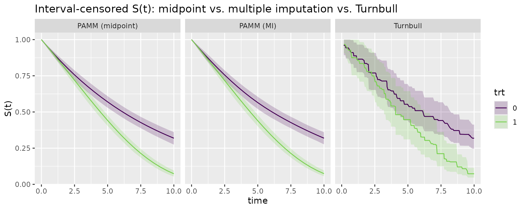

The over-confidence of the midpoint fit is easy to quantify. The ratio below is MI interval width / midpoint interval width, so values above one mean that proper MI gives wider intervals:

# MI-CI-width / midpoint-CI-width
summary((surv_mi$surv_upper  - surv_mi$surv_lower) / 
        (surv_mid$surv_upper - surv_mid$surv_lower))

##    Min. 1st Qu.  Median    Mean 3rd Qu.    Max.     NAs 
##  0.9452  0.9981  1.0474  1.0401  1.0583  1.2835       2

The effect is more visible on the hazard scale, which depends directly on exact event timing which interval censoring leaves more uncertain. Overlaying the two methods within each group shows the MI hazard bands enveloping the (over-confident) midpoint-based bands, while the point estimates mostly agree:

haz_panels <- c("Hazard rate", "Hazard FMI", "Observed censoring")
haz_all <- bind_rows(
  mutate(hazard_mid, method = "PAMM (midpoint)"),
  mutate(hazard_mi,  method = "PAMM (MI)")) %>%
  mutate(trt = paste0("trt = ", trt),
    method = factor(method, levels = c("PAMM (midpoint)", "PAMM (MI)")),
    panel = factor("Hazard rate", levels = haz_panels))

# true conditional hazards from the data-generating log-hazard
tgrid <- seq(0, 10, by = 0.1)
haz_true <- bind_rows(
  data.frame(tend = tgrid, trt = "trt = 0", hazard = exp(-2.2)),
  data.frame(tend = tgrid, trt = "trt = 1", hazard = exp(-2.2 + 0.15 * tgrid))) %>%
  mutate(panel = factor("Hazard rate", levels = haz_panels))

haz_fmi <- haz_fmi %>%
  mutate(panel = factor(panel, levels = haz_panels))

censor_panel <- icd %>%
  mutate(
    trt = paste0("trt = ", trt),
    panel = factor("Observed censoring", levels = haz_panels),
    kind = case_when(
      L == R ~ "Exact",
      is.infinite(R) ~ "Right-censored",
      TRUE ~ "Interval"
    ),
    xmin = pmax(L, 0),
    xmax = pmin(ifelse(is.infinite(R), 10, R), 10)
  ) %>%
  group_by(trt) %>%
  arrange(xmin, xmax, .by_group = TRUE) %>%
  mutate(subject = row_number()) %>%
  ungroup()

ggplot() +
  geom_stepribbon(data = haz_all,
    aes(x = tend, ymin = ci_lower, ymax = ci_upper, fill = method),
    alpha = 0.3, color = NA) +
  geom_step(data = haz_all,
    aes(x = tend, y = hazard, color = method)) +
  geom_line(data = haz_true, aes(x = tend, y = hazard), inherit.aes = FALSE,
    color = "gold", alpha = 0.5, linewidth = 0.9, linetype = 2) +
  geom_segment(data = filter(censor_panel, kind != "Exact"),
    aes(x = xmin, xend = xmax, y = subject, yend = subject),
    inherit.aes = FALSE, color = "grey35", alpha = 0.22, linewidth = 0.25) +
  geom_point(data = filter(censor_panel, kind == "Exact"),
    aes(x = xmin, y = subject),
    inherit.aes = FALSE, color = "grey10", alpha = 0.5, size = 0.45) +
  geom_step(data = haz_fmi, aes(x = tend, y = fmi),
    inherit.aes = FALSE, color = "black", linewidth = 0.8) +
  facet_grid(panel ~ trt, scales = "free_y") +
  scale_color_viridis_d(end = 0.5, aesthetics = c("colour", "fill"), option = "C") +
  labs(x = "time", y = NULL, color = NULL, fill = NULL,
    title = "Conditional hazard rate and hazard-scale FMI\n(true rates in gold)")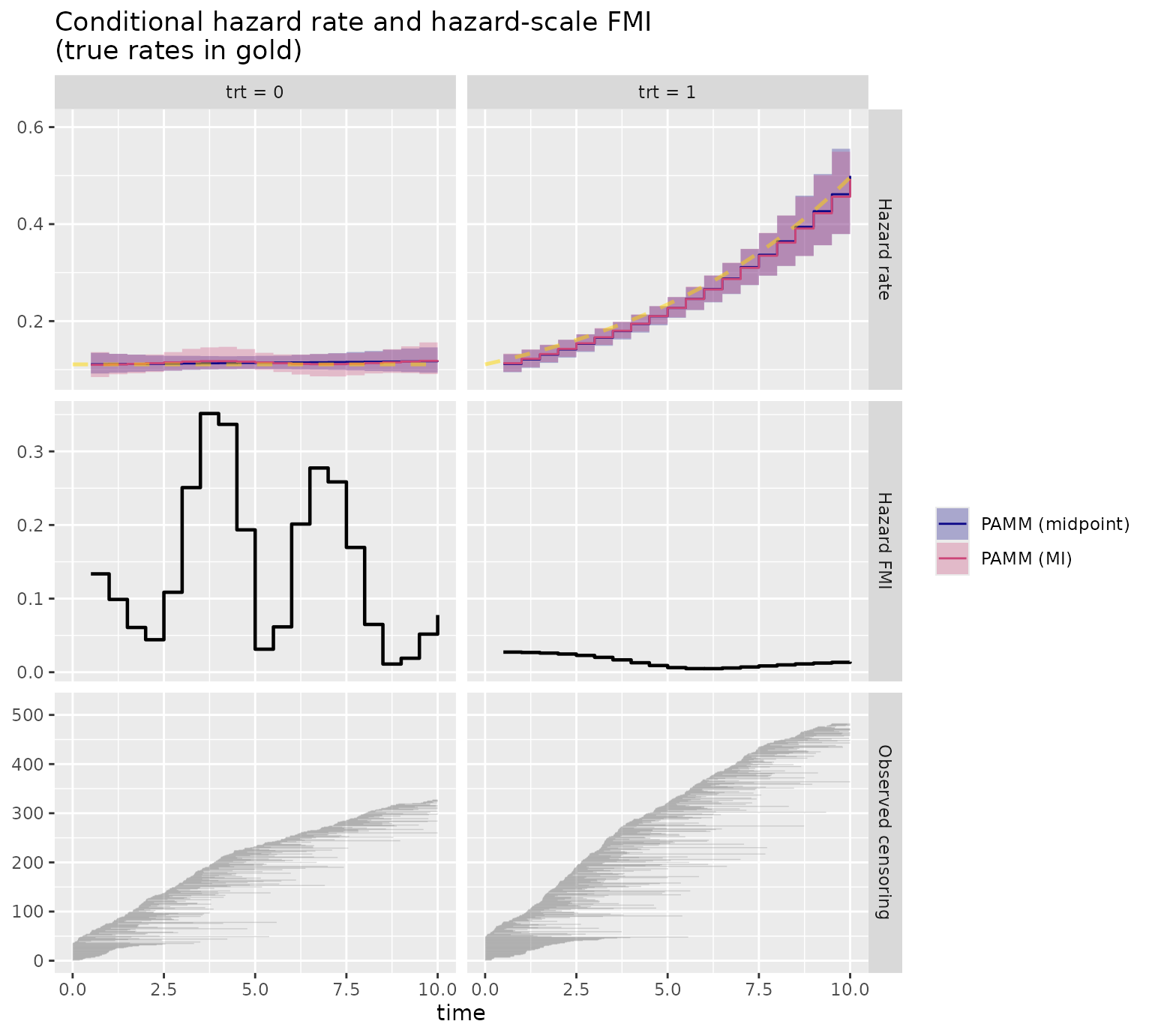

The true rates (gold) are tracked closely across the whole range – the constant trt = 0 hazard and the rising trt = 1 hazard are both recovered well. The midpoint and MI point estimates nearly coincide, consistent with midpoint giving reasonable point estimates but over-confident intervals; the MI bands are visibly wider throughout. The middle row shows where interval censoring bites on the hazard scale: high FMI means that most uncertainty in the local hazard estimate comes from not observing exact event times. The pattern is time-local, rather than a single model-wide number, because the event-time ambiguity matters most where the interval-censored observations leave the hazard shape weakly pinned down. The bottom row shows the observed censoring pattern itself: each horizontal line is one subject’s observed interval (right-censored observations are drawn up to the analysis horizon), and exact observations would appear as points.

The hazard interval-width ratio uses the same format as the survival calculation:

# MI-CI-width / midpoint-CI-width
summary((hazard_mi$ci_upper  - hazard_mi$ci_lower) /
        (hazard_mid$ci_upper - hazard_mid$ci_lower))

##    Min. 1st Qu.  Median    Mean 3rd Qu.    Max. 
##  0.9479  0.9830  1.0498  1.1451  1.2659  1.7150

So the imputation uncertainty inflates the hazard intervals more than the survival intervals: $S(t)$ aggregates the hazard over time and the group-level survival stays fairly well identified, whereas the hazard itself is tied directly to exact event times, which interval censoring leaves uncertain (cf. the large fraction of missing information reported by summary() above).
The same machinery is available for add_cumu_hazard().

Sparse inspection schedules: iterated MI

By default all m imputations are drawn from the single midpoint-initialised fit (“one-step” MI). When the inspection intervals are narrow relative to the time scale this is unbiased, but with wide gaps (mean gap of the order of a third of the follow-up) the initialiser’s midpoint bias leaks into the imputations: early-time survival is over-estimated, and – because the pooled standard errors remain honest – coverage deteriorates as $n$ grows.

The remedy is iter: with iter = k, each imputation chain alternates imputation and re-fitting on its own completed data $k$ times, so later imputations come from fits whose dependence on the initialiser is progressively attenuated (a chained-MI scheme in the spirit of poor man’s data augmentation (Wei and Tanner 1990) and the maxit iterations of mice (van Buuren and Groothuis-Oudshoorn 2011)).

fit_sparse <- pamm_ic(
  Surv(L, R, type = "interval2") ~ trt,
  data          = icd,
  model_formula = ped_status ~ trt + s(tend, by = trt),
  cut           = seq(0, 10, by = 0.5),
  m             = 20,
  iter          = 3   # recommended for sparse panels
)

Recommendation (from the package’s Monte Carlo benchmark, 500 replications per cell): keep the default iter = 1 for densely inspected data; use iter = 3 for sparse panels – it removes most of the early-time survival bias (iter = 5 essentially all of it, with bias shrinking roughly geometrically) at a fit cost roughly linear in iter. Two caveats from the same benchmark:

the hazard near sharp peaks remains attenuated under sparse inspection no matter how many iterations are used – with wide intervals that peak information is genuinely lost, not just imputed badly; and
with flexible time-varying-effect terms and small samples, iterating can occasionally amplify a weakly identified chain into a degenerate fit with vacuous intervals. pamm_ic() flags such chains with a warning (and in $unstable_chains); if it fires, inspect the affected fits and consider a less flexible model_formula or fewer iterations.

Competing risks

With $K$ competing causes, pamm_ic_cr() imputes the event time from a fitted cause-specific PAMM while retaining observed event causes. (It accepts the same iter argument as pamm_ic(), with the same sparse-panel recommendation.) This is the usual competing-risks interval-censoring setup: the cause is known at detection, but the event time is only known to lie in $(L, R]$ . If an event cause is explicitly missing (NA), pamm_ic_cr() can also sample the cause from the fitted cause-specific hazards at the imputed time. Each completed data set is then re-fit as a cause-specific PAMM, and cumulative incidence functions are obtained from those hazards with add_cif(). Note that this targets cause-specific hazards (and CIFs derived from them), and so differs from Delord and Génin (2016), who develop MI for interval-censored competing risks in the subdistribution-hazard (Fine–Gray) framework; the scheme here is the cause-specific analogue. Because we impute from a cause-specific model and analyse with one, the imputation and analysis models are congenial.

How event times are imputed when cause is known

For a subject known to fail from cause $k$ in $(L, R]$ , the correct conditional density of the event time is the cause- $k$ sub-density, restricted to the interval, $p(t \mid L < T \le R,\ \text{cause}=k) \;\propto\; f_k(t) = h_k(t)\,S(t), \qquad S(t) = \exp\!\Big(-\textstyle\int_0^t h_\bullet(u)\,du\Big),$ where $h_\bullet = \sum_j h_j$ is the all-cause hazard. The all-cause hazard is unavoidable here: to fail from cause $k$ at $t$ , the subject must first survive all causes up to $t$ (hence the all-cause survival $S$ ) and then fail from cause $k$ (hence $h_k$ ). Drawing instead from a “cause- $k$ -only” law $h_k(t)\exp(-\int h_k)$ would be the classic net/latent-time error – it ignores that a competing cause may remove the subject before $t$ , biasing imputed times too late.

The all-cause conditional CDF inverts in closed form on the piecewise grid (it is just the single-event sampler applied to $S = \exp(-H_\bullet)$ ), whereas $f_k(t) = h_k(t)S(t)$ has no equally clean inverse. So pamm_ic_cr() uses the all-cause conditional only as an easy-to-invert proposal and then accepts the draw with probability $h_k(t)/h_\bullet(t) \le 1$ . The accepted draws are proportional to (proposal) $\times$ (acceptance) $= h_\bullet(t)S(t)\cdot h_k(t)/h_\bullet(t) \propto h_k(t)S(t) = f_k(t)$ – exactly the target; the $h_\bullet$ cancels. The cause itself is not re-sampled in this known-cause case. For an unknown event cause (NA in the cause column), the same machinery is read the other way: the time is drawn from the all-cause conditional and the cause is then sampled with probability $h_k(t)/h_\bullet(t)$ , the same hazard / total_hazard ratio used to build CIF increments in add_cif().

Two consequences are worth noting:

If the cause-specific hazards are proportional ( $h_k/h_\bullet$ constant over time) the acceptance is uniform and the all-cause conditional already equals the cause- $k$ conditional – the rejection step is a no-op. It only matters when the cause mix shifts over follow-up (e.g. one cause dominates early, another late), which is exactly when cause- $k$ times need to be re-weighted.
For a rare cause $h_k/h_\bullet$ is small everywhere, so acceptance is low; the sampler caps the number of tries and errors if it cannot accept a valid proposal. For strongly imbalanced causes a direct inversion of the cause- $k$ sub-cumulative would be more robust – a possible refinement.

Example

To make the estimand visible, we simulate a small competing-risks data set with two genuinely different causes: cause 1 dominates early and decreases over time, whereas cause 2 rises later and is more common under treatment. The target estimands are the cause-specific CIFs $F_k(t \mid x) = P(T \le t, J = k \mid x)$ .

There is no direct survival::survfit() analogue of Turnbull’s estimator for interval-censored competing-risk CIFs. Since this is simulated data, however, we can use the latent exact event times to compute an oracle nonparametric Aalen-Johansen estimate and check whether the interval-censored MI fit recovers the same CIFs.

set.seed(4)
cr_cut <- seq(0, 10, by = 0.1)
cr_exact <- data.frame(trt = rbinom(700, 1, 0.5) |> as.factor()) |>
  sim_cr_piecewise(cut = cr_cut, max_time = 10)
icd_cr <- add_inspections(cr_exact, rate = 1.3, max_time = 10)
icd_cr$cause <- factor(icd_cr$cause)

fit_cr <- pamm_ic_cr(
  Surv(L, R, type = "interval2") ~ trt,
  cause = "cause",
  model_formula = ped_status ~ cause * trt + s(tend, by = cause, k = 6),
  cut = seq(0, 10, by = 0.5),
  data = icd_cr,
  m = 20
)
summary(fit_cr)

## Pooled PAMM summary (multiple imputation for interval-censored data)
## 
## Task           : competing risks 
## Family         : poisson 
## Model          : ped_status ~ cause * trt + s(tend, by = cause, k = 6) 
## Imputations    : 20 (proper) 
## Subjects       : 700 ( 501 interval/left-censored ); PED rows per fit: 17168 
## 
## Parametric coefficients (Rubin-pooled estimates & SEs, median-p):
##             Estimate Std. Error z value Pr(>|z|)    
## (Intercept)  -2.7972     0.0833  -33.58  < 2e-16 ***
## cause2       -0.7213     0.1428   -5.05  4.3e-07 ***
## trt1          0.0179     0.1243    0.14     0.89    
## cause2:trt1   0.9543     0.1844    5.17  2.2e-07 ***
## ---
## Signif. codes:  0 '***' 0.001 '**' 0.01 '*' 0.05 '.' 0.1 ' ' 1
## 
## Approximate significance of smooth terms (mean edf, median-p over imputations):
##                 edf Ref.df statistic p-value    
## s(tend):cause1 1.84   2.27      13.8  0.0018 ** 
## s(tend):cause2 1.01   1.01      66.6  <2e-16 ***
## ---
## Signif. codes:  0 '***' 0.001 '**' 0.01 '*' 0.05 '.' 0.1 ' ' 1
## 
## Fraction of missing information (FMI):
## Parametric coefficients:
##               FMI
## (Intercept) 0.003
## cause2      0.002
## trt1        0.002
## cause2:trt1 0.001
## 
## Smooth terms (five-number summaries over training PED rows):
##                  Min    Q1 Median    Q3   Max
## s(tend):cause1 0.051 0.102  0.543 0.822 0.822
## s(tend):cause2 0.014 0.026  0.493 0.955 0.955
## 
## Standard errors include within- + between-imputation variance (Rubin's rules);
## p-values are medians over imputations.

ped_cr <- as_ped(
  transform(icd_cr, time = pmin(true_time, 10), status = cause),
  Surv(time, status) ~ trt,
  cut = seq(0, 10, by = 0.5)
)
nd_cr <- make_newdata(
  ped_cr,
  tend = unique(tend),
  cause = levels(icd_cr$cause)[-1],
  trt = unique(trt)
) |>
  group_by(cause, trt)
cif_cr <- add_cif(nd_cr, fit_cr, nsim = 150)

aj_cr <- survfit(
  Surv(time, factor(cause, levels = c(0, 1, 2))) ~ trt,
  data = cr_exact
) |>
  aj_cif_df()
cif_lines <- bind_rows(
  transmute(cif_cr, tend, trt, cause, cif, method = "PAMM (MI)"),
  aj_cr
)
cif_lines$method <- factor(
  cif_lines$method,
  levels = c("PAMM (MI)", "Aalen-Johansen (true times)")
)

ggplot(cif_lines, aes(x = tend, y = cif, color = cause)) +
  geom_ribbon(data = cif_cr,
    aes(ymin = cif_lower, ymax = cif_upper, fill = cause),
    alpha = 0.18, color = NA) +
  geom_line(aes(linetype = method), linewidth = 0.8) +
  scale_color_viridis_d(end = 0.5, aesthetics = c("colour", "fill"), option = "C") +
  scale_linetype_manual(values = c("solid", "22")) +
  facet_grid(~ trt) +
  labs(x = "time", y = "CIF", color = "cause", fill = "cause", linetype = NULL,
    title = "Interval-censored competing-risk CIFs\nwith oracle Aalen-Johansen benchmark")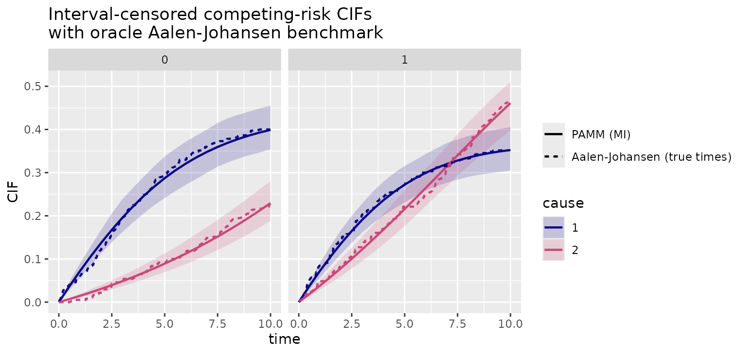

The dashed Aalen-Johansen curves use the simulated exact event times and are therefore an oracle reference, not an estimator available in a real interval-censored data set. They are useful here because they target the same CIFs as add_cif(). The MI curves track the oracle well: cause 1 contributes more early failures, while cause 2 accumulates later and more strongly in the treated group. This example is deliberately small so the vignette remains quick to render; for an analysis use a larger m and more posterior draws in add_cif().

Notes and limitations

The interval cut-points are fixed once and shared across all imputations; this is required for the imputations to be poolable.
The imputation-model coefficients are drawn from their posterior before each imputation (“proper” MI); this is what makes the pooled intervals calibrated.
Recurrent-event and general multi-state interval censoring are not yet supported: imputing one transition time changes the at-risk window for the next, so the imputations must be drawn jointly along each subject’s path – a planned extension.

References

Anderson-Bergman, Clifford. 2017. “icenReg: Regression Models for Interval Censored Data in R.” Journal of Statistical Software 81 (12): 1–23. https://doi.org/10.18637/jss.v081.i12.

Bebchuk, Judith D., and Rebecca A. Betensky. 2000. “Multiple Imputation for Simple Estimation of the Hazard Function Based on Interval Censored Data.” Statistics in Medicine 19 (3): 405–19. https://doi.org/10.1002/(SICI)1097-0258(20000215)19:3<405::AID-SIM799>3.0.CO;2-1.

Bolt, Matthew A., Samantha MaWhinney, Jack W. Pattee, Kristine M. Erlandson, David B. Badesch, and Ryan A. Peterson. 2022. “Inference Following Multiple Imputation for Generalized Additive Models: An Investigation of the Median p-Value Rule.” BMC Medical Research Methodology 22: 148. https://doi.org/10.1186/s12874-022-01613-w.

Delord, Marc, and Emmanuelle Génin. 2016. “Multiple Imputation for Competing Risks Regression with Interval-Censored Data.” Journal of Statistical Computation and Simulation 86 (11): 2217–28. https://doi.org/10.1080/00949655.2015.1100633.

Pan, Wei. 2000. “A Multiple Imputation Approach to Cox Regression with Interval-Censored Data.” Biometrics 56 (1): 199–203. https://doi.org/10.1111/j.0006-341X.2000.00199.x.

Rubin, Donald B. 1987. Multiple Imputation for Nonresponse in Surveys. John Wiley & Sons. https://doi.org/10.1002/9780470316696.

van Buuren, Stef, and Karin Groothuis-Oudshoorn. 2011. “mice: Multivariate Imputation by Chained Equations in R.” Journal of Statistical Software 45 (3): 1–67. https://doi.org/10.18637/jss.v045.i03.

Wei, Greg C. G., and Martin A. Tanner. 1990. “A Monte Carlo Implementation of the EM Algorithm and the Poor Man’s Data Augmentation Algorithms.” Journal of the American Statistical Association 85 (411): 699–704. https://doi.org/10.1080/01621459.1990.10474930.

pammtools

2026-06-17