Defining a new backend: gradient boosting with xgboost

Show package setup

library(dplyr)
library(ggplot2)
theme_set(theme_bw())
library(survival)
library(mgcv)
library(xgboost)
library(pammtools)
Set1 <- RColorBrewer::brewer.pal(9, "Set1")

Why a new backend is cheap

The key idea behind PAMMs (Bender et al. 2018) is a data transformation: a time-to-event data set is split into the piece-wise exponential data (PED) format, and the hazard is then estimated by a Poisson regression with a log-interval-length offset. The default estimation engine in pammtools is mgcv::gam, but the reduction to Poisson regression means that any learner that can do count/Poisson regression with an offset can serve as a PAMM backend.

To make a backend a first-class citizen, pammtools abstracts every model behind a small internal interface and builds all of its post-processing on top of it. Two primitives are enough for point estimates and simulation-based intervals of every derived quantity:

get_hazard(object, newdata) — the point hazard (a numeric vector);
sim_hazard(object, newdata, nsim) — a matrix of hazard draws from the model’s sampling distribution, used for the simulation-based intervals.

Analytic ("default"/"delta") intervals additionally need the coefficient triplet make_X() / get_coefs() / get_Vp(); a backend that does not provide them simply uses ci_type = "sim".

Everything else — add_hazard(), add_cumu_hazard(), add_surv_prob() (point estimates and intervals), and the geom_* plotting layers — is written against this interface. So to teach xgboost to act as a PAMM backend we only need to express it in these terms; the entire workflow then works unchanged.

As the example learner we use xgboost (Chen and Guestrin 2016) with its built-in objective = "count:poisson". Since a boosted tree ensemble has no coefficient covariance, we obtain uncertainty from a subject-level bootstrap ensemble (bagging): the point estimate is the bagged mean hazard, and confidence bands are percentiles across the ensemble members.

The backend

1. A ped becomes an xgboost data set. A ped already carries the bookkeeping we need in its attributes: intvars lists the internal interval columns, ped_status is the Poisson response, and offset is the log-interval-length. We keep tend as the time feature, drop the remaining internal columns and — the only trick — pass the PED offset as xgboost’s base_margin, so it plays the role of the Poisson offset.

xgb_feature_cols <- function(ped) {
  internal <- attr(ped, "intvars")
  keep <- intersect(c("cause", "transition"), names(ped))
  c("tend", setdiff(names(ped), setdiff(internal, keep)))
}

as_xgb_data <- function(ped) {
  features <- xgb_feature_cols(ped)
  x <- model.matrix(~ . - 1, data = as.data.frame(ped)[, features, drop = FALSE])
  d <- xgb.DMatrix(x, label = ped[["ped_status"]])
  setinfo(d, "base_margin", ped[["offset"]]) # PEM offset = log(interval length)
  d
}

2. Fitting = a bootstrap ensemble of boosters. We resample subjects (the id_var) with replacement and fit one booster per replicate. Setting base_score = 1 together with the offset means that at prediction time (where we supply no base_margin) the default margin is log(base_score) = 0, so predictions are the bare hazard exp(trees). We store the ensemble plus the features it expects; the object is a plain list of class pam_xgb.

xgb_pam <- function(ped, params = list(), nrounds = 200, nboot = 40, ...) {
  features <- xgb_feature_cols(ped)
  id_var   <- attr(ped, "id_var")
  X   <- model.matrix(~ . - 1, data = as.data.frame(ped)[, features, drop = FALSE])
  y   <- ped[["ped_status"]]
  off <- ped[["offset"]]
  feature_levels <- lapply(as.data.frame(ped)[, features, drop = FALSE], function(x) {
    if (is.factor(x)) {
      levels(x)
    } else if (is.character(x)) {
      sort(unique(x))
    } else {
      NULL
    }
  })
  rows_by_id <- split(seq_len(nrow(ped)), ped[[id_var]])
  params <- c(params, list(objective = "count:poisson", base_score = 1, nthread = 2))
  fit_rows <- function(rows) {
    d <- xgb.DMatrix(X[rows, , drop = FALSE], label = y[rows])
    setinfo(d, "base_margin", off[rows])
    xgb.train(params = params, data = d, nrounds = nrounds, verbose = 0, ...)
  }
  models <- lapply(seq_len(nboot), function(b) {
    fit_rows(unlist(rows_by_id[sample(names(rows_by_id), replace = TRUE)],
                    use.names = FALSE))
  })
  structure(
    list(models = models, orig_features = features,
         feature_levels = feature_levels,
         trafo_args = attr(ped, "trafo_args")),
    class = "pam_xgb")
}

3. Plugging into the pammtools interface. pammtools builds every derived quantity and its simulation-based confidence intervals from two per-model primitives, so all we implement are these two S3 methods:¹

get_hazard() returns the point hazard as a plain vector (here the bagged mean over the ensemble);
sim_hazard() returns a matrix of hazard draws (one column per draw). For our ensemble a “draw” is a bootstrap member, so we predict the feature matrix through every booster.

get_hazard.pam_xgb <- function(object, newdata, ...) {
  rowMeans(sim_hazard.pam_xgb(object, newdata))      # bagged point hazard
}

sim_hazard.pam_xgb <- function(object, newdata, nsim = NULL, ...) {
  xdf <- as.data.frame(newdata)[, object$orig_features, drop = FALSE]
  for (nm in names(object$feature_levels)) {
    if (!is.null(object$feature_levels[[nm]]) && nm %in% names(xdf)) {
      xdf[[nm]] <- factor(xdf[[nm]], levels = object$feature_levels[[nm]])
    }
  }
  X  <- model.matrix(~ . - 1, data = xdf)
  dm <- xgb.DMatrix(X)
  vapply(object$models, function(m) predict(m, dm), numeric(nrow(X))) # rows x members
}

That is the whole backend. add_hazard(), add_cumu_hazard(ci_type = "sim") and add_surv_prob(ci_type = "sim") now work for pam_xgb objects, returning point estimates and bootstrap intervals, and the geom_* layers plot them, all for free. The very same engine also drives add_cif() (competing risks) and add_trans_prob() (multistate) from these two primitives — a backend that keeps the cause/transition indicator among its features gets those for free too.

Example 1: recovering a known hazard, with uncertainty

We simulate from a known hazard with sim_pexp and transform to PED with as_ped, exactly as for a standard PAMM. Passing cut to as_ped fixes a modest interval grid (here 20 intervals), which keeps the boosters fast to fit.

set.seed(2024)
n  <- 2000
df <- data.frame(x1 = runif(n, -2, 2), x2 = runif(n, 0, 4))
# true log-hazard: smooth baseline + linear x1 + linear x2
f_true <- function(t, x1, x2) -2.2 + 0.5 * sin(0.8 * t) - 0.4 * x1 + 0.25 * x2
sim_df <- sim_pexp(~ -2.2 + 0.5 * sin(0.8 * t) - 0.4 * x1 + 0.25 * x2, df,
                   cut = seq(0, 6, by = 0.1))
ped <- as_ped(sim_df, Surv(time, status) ~ x1 + x2, cut = seq(0, 6, by = 0.3))

We fit the boosted PAMM with xgb_pam() and, for comparison, a standard GAM-based PAMM.

xgb_fit <- xgb_pam(ped,
  params  = list(eta = 0.1, max_depth = 3, min_child_weight = 20,
                 subsample = 0.7, colsample_bytree = 0.8),
  nrounds = 200, nboot = 40)

pam <- gam(ped_status ~ s(tend) + x1 + s(x2), data = ped,
  family = poisson(), offset = offset)

For prediction we build a grid with make_newdata and add the hazard with the same add_hazard() call for both models — the boosted one is served by our get_hazard.pam_xgb method, returning bootstrap confidence bands.

nd <- ped %>% make_newdata(tend = unique(tend), x1 = c(-1, 1), x2 = c(2))

haz <- bind_rows(
  nd %>% group_by(x1, x2) %>% add_hazard(xgb_fit, ci_type = "sim") %>% mutate(method = "xgboost"),
  nd %>% group_by(x1, x2) %>% add_hazard(pam, ci = TRUE)           %>% mutate(method = "gam (PAMM)")
) %>%
  mutate(truth = exp(f_true(tend, x1, x2)),
         profile = paste0("x1 = ", x1))

ggplot(haz, aes(x = tend)) +
  geom_stepribbon(aes(ymin = ci_lower, ymax = ci_upper, fill = method), alpha = 0.2) +
  geom_stephazard(aes(y = hazard, col = method)) +
  geom_line(aes(y = truth), lty = 2) +
  facet_wrap(~ profile) +
  scale_color_manual(values = c("xgboost" = Set1[2], "gam (PAMM)" = Set1[1])) +
  scale_fill_manual(values  = c("xgboost" = Set1[2], "gam (PAMM)" = Set1[1])) +
  labs(y = "hazard", col = "", fill = "",
       title = "Estimated hazard (95% CI) vs. truth (dashed)")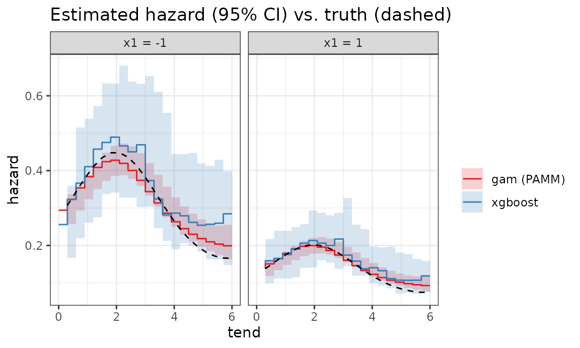

Both backends recover the baseline shape and the covariate effects; the GAM is smooth by construction, while the boosted hazard is piece-wise constant. The bootstrap bands of the boosted fit are comparable to the GAM’s Bayesian intervals.

Survival probabilities come from the same machinery via add_surv_prob() with ci_type = "sim" — no manual cumulative sums:

surv <- nd %>%
  group_by(x1, x2) %>%
  add_surv_prob(xgb_fit, ci_type = "sim") %>%
  ungroup() %>%
  group_by(x1, x2) %>%
  mutate(truth = exp(-cumsum(exp(f_true(tend, x1, x2)) * (tend - lag(tend, default = 0))))) %>%
  ungroup() %>%
  mutate(profile = paste0("x1 = ", x1))

ggplot(surv, aes(x = tend)) +
  geom_ribbon(aes(ymin = surv_lower, ymax = surv_upper), alpha = 0.2, fill = Set1[2]) +
  geom_line(aes(y = surv_prob), col = Set1[2]) +
  geom_line(aes(y = truth), lty = 2) +
  facet_wrap(~ profile) +
  labs(y = "survival probability",
       title = "Boosted survival probability (95% CI) vs. truth (dashed)")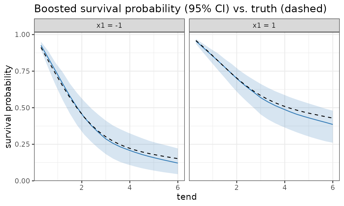

Example 2: a time-varying effect, recovered automatically

Because tend is just another feature, the trees can model tend-by-covariate interactions, i.e. time-varying effects, without us specifying them. Here the effect of x1 grows over time, β(t) = 0.1 + 0.25 t — a clear violation of proportional hazards.

set.seed(7)
n   <- 4000
df2 <- data.frame(x1 = runif(n, -1.5, 1.5), x2 = runif(n, -1, 1))
beta_true <- function(t) 0.1 + 0.25 * t
f2_true   <- function(t, x1, x2) -2.0 + 0.3 * sin(0.8 * t) + beta_true(t) * x1 + 0.3 * x2
sim2 <- sim_pexp(~ -2.0 + 0.3 * sin(0.8 * t) + (0.1 + 0.25 * t) * x1 + 0.3 * x2, df2,
                 cut = seq(0, 6, by = 0.1))
ped2 <- as_ped(sim2, Surv(time, status) ~ x1 + x2, cut = seq(0, 6, by = 0.3))

xgb2 <- xgb_pam(ped2,
  params  = list(eta = 0.1, max_depth = 3, min_child_weight = 20,
                 subsample = 0.7, colsample_bytree = 0.8),
  nrounds = 200, nboot = 40)

The estimated hazard for x1 ∈ {-1, 0, 1} shows the gap between the curves widening over time, tracking the truth:

nd2 <- ped2 %>% make_newdata(tend = unique(tend), x1 = c(-1, 0, 1), x2 = c(0))
haz2 <- nd2 %>%
  group_by(x1, x2) %>%
  add_hazard(xgb2, ci_type = "sim") %>%
  ungroup() %>%
  mutate(truth = exp(f2_true(tend, x1, x2)), x1 = factor(x1))

ggplot(haz2, aes(x = tend, col = x1, fill = x1)) +
  geom_stepribbon(aes(ymin = ci_lower, ymax = ci_upper), alpha = 0.2, col = NA) +
  geom_stephazard(aes(y = hazard)) +
  geom_line(aes(y = truth), lty = 2) +
  scale_color_manual(values = Set1[c(1, 3, 2)]) +
  scale_fill_manual(values  = Set1[c(1, 3, 2)]) +
  labs(y = "hazard", col = "x1", fill = "x1",
       title = "Time-varying effect: hazard (95% CI) vs. truth (dashed)")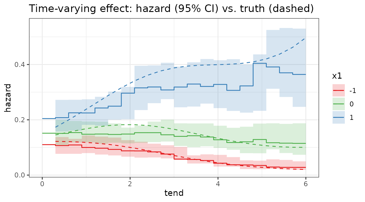

We can read off the estimated time-varying log-hazard ratio β(t) = log h(x1 = 1) / h(x1 = 0) directly from the ensemble (one ratio trajectory per member), and it recovers the true linear-in-time effect with honest uncertainty:

feat_mat <- function(d) model.matrix(~ . - 1,
  as.data.frame(d)[, xgb2$orig_features, drop = FALSE])
grid <- ped2 %>% make_newdata(tend = unique(tend), x1 = c(0, 1), x2 = c(0))
H1 <- vapply(xgb2$models, function(m) predict(m, xgb.DMatrix(feat_mat(filter(grid, x1 == 1)))),
             numeric(length(unique(grid$tend))))
H0 <- vapply(xgb2$models, function(m) predict(m, xgb.DMatrix(feat_mat(filter(grid, x1 == 0)))),
             numeric(length(unique(grid$tend))))
beta_hat <- data.frame(
  tend  = sort(unique(grid$tend)),
  est   = rowMeans(log(H1 / H0)),
  lower = apply(log(H1 / H0), 1, quantile, 0.025, type = 6),
  upper = apply(log(H1 / H0), 1, quantile, 0.975, type = 6))

ggplot(beta_hat, aes(x = tend)) +
  geom_ribbon(aes(ymin = lower, ymax = upper), alpha = 0.2, fill = Set1[2]) +
  geom_line(aes(y = est), col = Set1[2]) +
  geom_line(aes(y = beta_true(tend)), lty = 2) +
  labs(y = expression(beta(t)),
       title = expression("Estimated time-varying log-hazard ratio " * beta(t) * " (95% CI) vs. truth"))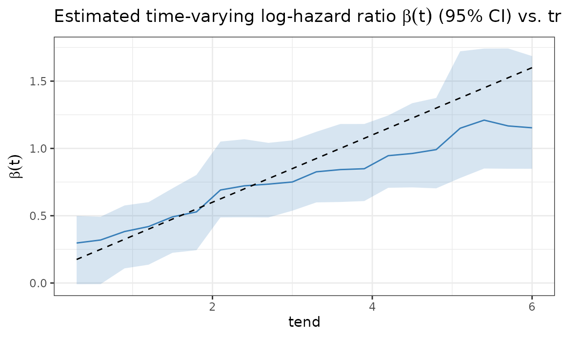

Example 3: competing risks with the same backend

This last example additionally needs etm for the fourD data. We reuse the same xgb_pam() helper, but now fit it to a stacked cause-specific PED. Because the cause indicator is just another feature, add_cif() can recover cause-specific cumulative incidence curves from the same backend interface.

data("fourD", package = "etm")

set.seed(2025)
cut <- sample(fourD$time, 100)

ped_cr <- fourD %>%
  select(id, time, status, sex, age) %>%
  as_ped(Surv(time, status) ~ ., id = "id", cut = cut) %>%
  mutate(cause = as.factor(cause))

xgb_cr <- xgb_pam(
  ped_cr,
  params = list(
    eta = 0.1, max_depth = 3, min_child_weight = 20,
    subsample = 0.7, colsample_bytree = 0.8
  ),
  nrounds = 200, nboot = 40
)

For the CIF we create a prediction grid over time, cause, and sex and then use the same add_cif() call as for a standard PAMM:

nd_cr <- ped_cr %>%
  make_newdata(tend = unique(tend), cause = unique(cause), sex = unique(sex)) %>%
  group_by(cause, sex) %>%
  add_cif(xgb_cr, nsim = length(xgb_cr$models))

ggplot(nd_cr, aes(x = tend, y = cif)) +
  geom_line(aes(col = cause)) +
  geom_ribbon(
    aes(ymin = cif_lower, ymax = cif_upper, fill = cause),
    alpha = 0.2
  ) +
  facet_wrap(~ sex, labeller = label_both) +
  labs(
    y = "cumulative incidence",
    col = "cause",
    fill = "cause",
    title = "Cause-specific CIFs from the xgboost backend"
  )

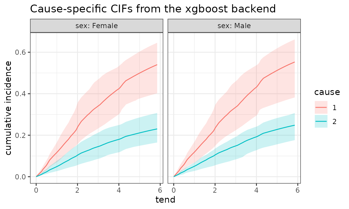
The only difference to the standard competing-risks vignette is the fitting engine. The prediction pipeline, including the bootstrap uncertainty bands, is still driven entirely by get_hazard() and sim_hazard().

Wrap-up

A usable xgboost backend for PAMMs took four short functions: two helpers (as_xgb_data, xgb_pam) and two S3 methods (get_hazard.pam_xgb, sim_hazard.pam_xgb) expressed against pammtools’ model interface. Everything else — make_newdata, add_hazard, add_cumu_hazard, add_surv_prob, the geom_* layers and the bootstrap confidence intervals — came for free.

A caveat on inference: the bootstrap bands capture the sampling variability of the ensemble. Like for any flexible learner, they do not reflect the approximation bias of the trees, so they can be optimistic in regions where the ensemble is systematically off — visible here at the end of follow-up, where data are sparse and the estimated time-varying effect β(t) lags behind the truth. The same recipe extends to tuning/cross-validation and to competing risks (stack cause-specific PEDs and use the same offset trick), with no changes to pammtools itself.

References

Bender, Andreas, Andreas Groll, and Fabian Scheipl. 2018. “A Generalized Additive Model Approach to Time-to-Event Analysis.” Statistical Modelling 18 (3-4): 299–321. https://doi.org/10.1177/1471082X17748083.

Chen, Tianqi, and Carlos Guestrin. 2016. “XGBoost: A Scalable Tree Boosting System.” Proceedings of the 22nd ACM SIGKDD International Conference on Knowledge Discovery and Data Mining (KDD ’16) (New York, NY, USA), 785–94. https://doi.org/10.1145/2939672.2939785.

For a second worked example of these two methods — defining get_hazard()/sim_hazard() for a Bayesian brms model, where a “draw” is a posterior sample rather than a bootstrap member — see the Bayesian baseline PAMMs article.↩︎